Neutrinos & Neutrino Oscillations - Thesis

2. Neutrinos & Neutrino Oscillations

The existence of a light, weakly-interacting neutral particle was first suggested by Wolfgang Pauli in 1930 to explain the energy spectrum observed for electrons/positrons emitted in beta decays. Although not universally popular at first (even Pauli himself was sceptical) the idea eventually became widely accepted, but it was not until 1956 that the first experimental detection of “neutrinos” was made [1].

In the decades which followed discovery, their use in experiments was as probes of other physics. For example, the study of solar neutrinos was mainly motivated by understanding the fusion processes present in the Sun. Likewise, accelerator-based neutrino beams were made to study the workings of the weak force at lower energies than would be possible with electromagnetically or strongly interacting particles.

It wasn’t until observation of the solar and atmospheric neutrino problems, and the eventual discovery of neutrino oscillations, that neutrinos became of interest in their own right.

2.1. Neutrino States

The leptons, like all matter particles in the Standard Model, exhibit the peculiar feature that the states in which they undergo charged-current weak interactions, “flavour states”, are not mass eigenstates1This is unlike the electromagnetic and strong interactions, whose interaction states are mass eigenstates.. Instead the three flavour states are a superposition, or mixture, of the three mass states [2].

Experimentally we have the freedom to define the reference point from which the flavour states are measured. Conventionally in quarks, we define the flavour states in terms of the up-type quarks, such that all the mixing occurs in the down-type quarks. Similarly in neutrinos, the convention is to define the flavour states in terms of the charged leptons with all the mixing confined to the neutrinos. There is good reason for this choice: the fact that neutrinos interact only weakly and that the differences between their masses are tiny, make it impossible to measure which mass state has been created.

One will sometimes find one or other of the flavour/mass states being described as the “physical” states (usually mass in quarks and flavour in neutrinos) but such a description is misleading. It is the measurement being made which determines which states are important, and any perception that one set is more “real” than another is simply an artefact of the view the experimenter has.

It is natural to assume that like the other fermions each neutrino flavour ν_α has an anti-matter equivalent ν_α, i.e. that they are Dirac particles. However because of their neutral charge it is possible that neutrinos could be Majorana particles. If this were to be the case then neutrinos would be their own anti-particles and they could have both Majorana and Dirac masses.

Today it is thought there are three neutrino flavour states which are defined by the charged lepton they interact with at charged-current weak vertices: ν_e, ν_μ and ν_τ. There are also three mass states ν₁, ν₂, ν₃ with masses m₁, m₂ and m₃ respectively:

The mass and flavour states are related by a mixing matrix:

(\begin{matrix} ν_{e} \\ ν_{μ} \\ ν_{τ} \end{matrix}) = (\begin{matrix} U_{e1} & U_{e2} & U_{e3} \\ U_{μ1} & U_{μ2} & U_{μ3} \\ U_{τ1} & U_{τ2} & U_{τ3} \end{matrix}) (\begin{matrix} ν_{1} \\ ν_{2} \\ ν_{3} \end{matrix})

(2.1)

This unitary matrix is known as the “Pontecorvo-Maki-Nakagawa-Sakata” matrix [3] [4]. The expression can also be inverted to express the mass states, i, in terms of the flavour states, α, highlighting the fact that they are both mixtures of each other:

ν_{i} = \underset{α}{Σ} {U*}_{αi} ν_{α}

(2.2)

It is convenient for experimental purposes to parametrise the PMNS matrix as the product of four sub-matrices [2]:

U_{PMNS} = (\begin{matrix} 1 & 0 & 0 \\ 0 & cos θ_{23} & sin θ_{23} \\ 0 & - sin θ_{23} & cos θ_{23} \end{matrix}) (\begin{matrix} cos θ_{13} & 0 & sin θ_{13} e^{-iδ} \\ 0 & 1 & 0 \\ - sin θ_{13} e^{-iδ} & 0 & cos θ_{13} \end{matrix}) (\begin{matrix} cos θ_{12} & sin θ_{12} & 0 \\ - sin θ_{12} & cos θ_{12} & 0 \\ 0 & 0 & 1 \end{matrix}) (\begin{matrix} e^{½ i α_{1}} & 0 & 0 \\ 0 & e^{½ i α_{2}} & 0 \\ 0 & 0 & 1 \end{matrix})

(2.3)

This parametrisation consists of three mixing angles (θ₁₂, θ₂₃ and θ₁₃) two Majorana CP-violating phases (α₁ and α₂) and one Dirac CP-violating phase (δ).

The value of the three mixing angles effectively determines the degree to which the mass and flavour states are mixed.

The phases α₁ and α₂ are only physically observable if neutrinos are Majorana particles. Even if they exist it will be very difficult to measure their values experimentally, but in either case they do not contribute at all to neutrino oscillations (so they will be neglected from here on in).

However the final phase δ, which is commonly referred to as δ_cp, is directly observable and, if its value is non-zero, represents the source of leptonic CP-violation which most strongly motivates our interest in oscillations. As can be seen in Equation 2.3 however, it only appears with terms of sinθ₁₃ so, regardless of the value of δ_cp, we also require θ₁₃ ≠ 0 for any CP-violating effects to exist.

2.2. Neutrino Oscillations

Neutrino oscillations is a phenomenon which occurs as a result of the mixing of neutrino flavour and mass states discussed above. Experimentally it is the observation of a change in the flavour composition of neutrinos as they travel away from their source.

When a neutrino is created, it is created by the weak force, and therefore exists in a weak (flavour) eigenstate. So the wavefunction describing a pure source of ν_α at creation looks like:

|ψ (0,0)〉 = |ν_{α}〉 = U_{α1} |ν_{1}〉 + U_{α2} |ν_{2}〉 + U_{α3} |ν_{3}〉

(2.4)

Later, after travelling a distance L through a vacuum the wavefunction becomes:

|ψ (L,t)〉 = U_{α1} |ν_{1}〉 e^{-i φ_{1}} + U_{α2} |ν_{2}〉 e^{-i φ_{2}} + U_{α3} |ν_{3}〉 e^{-i φ_{3}}

(2.5)

where, assuming a plane-wavefunction2Assuming plane-wavefunctions gives the same results as a more complete treatments in all but extreme cases [5]., each mass state has acquired a phase φ_i = E_it - |p_i|L. Since each of these states represents a different mass, the phases are also slightly different. So as the neutrinos travel away from the source, the mass states get out of phase with one another and the resulting interference means that the wavefunction evolves to contain components from all three flavour states. This can be seen from Equation 2.5 by substituting the mass states for their flavour mixtures from Equation 2.2:

\begin{matrix} |ψ (L,t)〉 & = (U_{α1} {U*}_{e1} e^{-i φ_{1}} + U_{α2} {U*}_{e2} e^{-i φ_{2}} + U_{α3} {U*}_{e3} e^{-i φ_{3}}) |ν_{e}〉 \\ + (U_{α1} {U*}_{μ1} e^{-i φ_{1}} + U_{α2} {U*}_{μ2} e^{-i φ_{2}} + U_{α3} {U*}_{μ3} e^{-i φ_{3}}) |ν_{μ}〉 \\ + (U_{α1} {U*}_{τ1} e^{-i φ_{1}} + U_{α2} {U*}_{τ2} e^{-i φ_{2}} + U_{α3} {U*}_{τ3} e^{-i φ_{3}}) |ν_{τ}〉 \end{matrix}

(2.6)

After travelling a distance L through a vacuum the neutrino wavefunction, which was initially pure ν_α, is now a mixture of all three neutrino types and the proportion of each flavour varies as the neutrinos travel. This is neutrino oscillations.

Expanding Equation 2.6 out and calculating an example probability gets cumbersome so we make the assumption, valid at the resolution of current experiments, that δ_cp is zero to simplify things. Then for a beam of initially pure ν_μ with energy E, the probability of a neutrino being a ν_e at a distance L from the source is:

\begin{matrix} P (ν_{μ} \to ν_{e}) = {sin}^{2} (θ_{23}) {sin}^{2} ({2θ}_{13}) {sin}^{2} ({Δm}^{2}_{32} Φ) + {cos}^{2} (θ_{23}) {sin}^{2} ({2θ}_{13}) {sin}^{2} ({Δm}^{2}_{21} Φ) \\ + cos (θ_{13}) sin ({2θ}_{12}) sin ({2θ}_{13}) sin ({2θ}_{23}) sin ({Δm}^{2}_{32} Φ) sin ({Δm}^{2}_{21} Φ) cos ({Δm}^{2}_{32} Φ) \end{matrix}

(2.7)

Where, for the sake of brevity:

Φ = \frac{L}{4E}

(2.8)

and we meet for the first time the mass-splittings:

{Δm}^{2}_{ij} = {m_{i}}^{2} - {m_{j}}^{2}

(2.9)

We can plot this probability as a function of L/E (Figure 2.1), making the origin of the name “oscillations” more apparent.

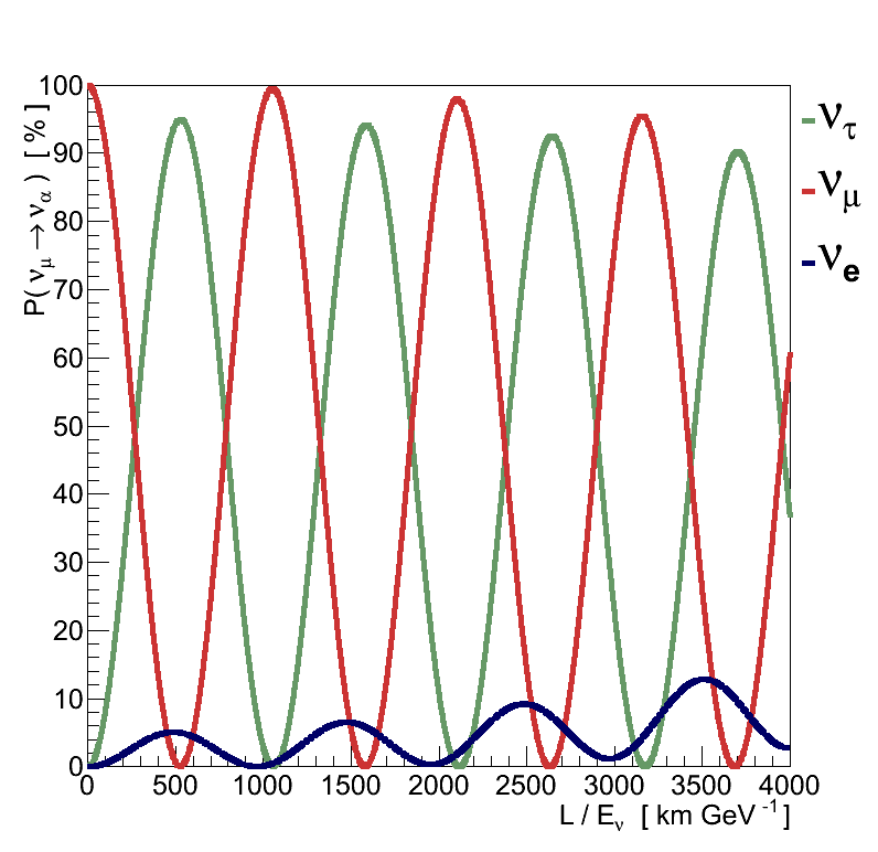
Figure 2.1: The detection probability of the three neutrino flavours from an initially pure ν_μ beam, as a function of L/E_ν (using values from Table 2.1). Over longer distances, or at lower energies, “beat” patterns emerge - the neutrinos essentially behave as three coupled oscillators. The fact that the ν_μ component can reach both 1 and 0 is a consequence of θ₂₃ = 45 °.

Oscillations are therefore a function of the three mixing angles, the distance travelled (often called the baseline) and the neutrino energy. They are also a function of the size of the differences between the mass states, Δm²_ij, which is unsurprising given that it is the differences in how the states propagate, and hence their phases, that cause the oscillations. There are three of these mass splittings but since:

{Δm}^{2}_{32} + {Δm}^{2}_{21} = {Δm}^{2}_{31}

(2.10)

there are only two which are independent. It is also worth emphasizing that it is only the differences between the masses which matter and neutrino oscillations are insensitive to the absolute scale of the three masses.

The Particle Data Group [2] provide a review of current world knowledge of the values of all the fundamental parameters that contribute to neutrino oscillations, which are summarised in Table 2.1.

Table 2.1: Current world knowledge of the neutrino oscillation parameters [2].
Parameter	Value
θ₁₂	33.9 ± 1.0 °
θ₂₃	39 ° < θ₂₃ < 51 °
θ₁₃	9.1 ± 0.6 °
Δm²₂₁	(7.50 ± 0.20) ×10^-5 eV²
\|Δm²₃₂\|	(2.32 ^+0.12_-0.08) ×10^-3 eV²
δ_cp	unknown

The equations above all apply to oscillations in a vacuum, however the situation is complicated further when a neutrino beam passes through matter. Because matter contains electrons but none of the other charged leptons/anti-leptons, ν_e have an additional interaction mode (CC forward scattering) available to them which is unavailable to the other neutrino flavours. This gives a larger effective mass to the ν_e component, which in turn affects the propagation of the associated states and hence the oscillations. The magnitude of the effect increases with the distance travelled in matter and the electron density encountered. Matter effects are not significant in the T2K experiment so won't be discussed in any more depth, but they are important in longer baseline experiments.

Finally, it is possible that there could be more than three neutrino flavour states, though the additional states would have to be “sterile”, i.e. not interact via the weak force, or it would conflict with other experimental evidence (the decay width of the Z⁰ [6], for example). If this were the case the mixing matrix would have to grow to accommodate it, and there may or may not be more neutrino mass states as well. However at present there is no convincing or consistent evidence to suggest that steriles exist [2].

2.3. Neutrino Masses

In the Standard Model neutrinos have always been treated as massless particles and it is only the discovery of neutrino oscillations which has given us any evidence to suggest otherwise.

The fact that any oscillations occur means that one of the Δm²_ij ≠ 0, implying that at least one of the neutrino masses must also be non-zero. In fact, since all of the mass splittings are measured to be non-zero at least two of the masses are required to be non-zero. However, as discussed in Section 2.2, oscillations are insensitive to the absolute values of the neutrino masses and can only observe the differences between them.

At present the masses have proven to be so small that they are inaccessible to current experiments. The end-point of tritium beta-decay in the Troitzk experiment sets the world's most stringent limit: m_{ν_e} < 2.05 eV at 95% CL [7]. Though it should be noted that the mass measured here, m_{ν_e}, is that of a flavour state, and therefore represents a combination of the three mass states it contains.

Even with the mass differences we can measure, thus far it has not been possible to determine the sign of Δm²₃₁. The two possibilities are referred to as the “normal” (Δm²₃₁ > 0) and “inverted” (Δm²₃₁ < 0) hierarchies, and amount to a choice between which of the mass states is largest:

\begin{matrix} Normal Hierarchy: & m_{3} > m_{2} > m_{1} \\ Inverted Hierarchy: & m_{2} > m_{1} > m_{3} \end{matrix}

(2.11)

The difficulty in determining the sign is essentially caused by the uncertainties on Δm²₃₂ and Δm²₃₁ being larger than the size of Δm²₂₁, and therefore the sign has a negligible effect on the oscillation probabilities compared to current experimental uncertainties. It is only matter effects in solar neutrino oscillations that have allowed us to determine the sign of Δm²₂₁.

2.4. Measuring Neutrino Oscillation Parameters

Equation 2.7 tells us that neutrino oscillations depend on the mixing angles, the mass splittings, the distance travelled and the neutrino energy. The mixing angles and mass splittings are properties of the Universe, we can't change them, we can only measure them. The distance travelled in a conventional accelerator-based oscillation experiment is a fixed quantity which we know.

The final parameter, the neutrino energy, is a property of the neutrino source - but that's an oversimplification. There is no practical way to create a mono-energetic neutrino source3There are options for creating mono-energetic neutrinos but none of them are practical. Pion decay at rest would provide a mono-energetic ν_μ source, but their ∼30 MeV energy would be too low for ν_μ CC interactions. Alternatively, Z⁰ decay at rest would make an interesting neutrino source. Around 20% would decay to give an even mix of all six neutrinos and anti-neutrinos at 45.6 GeV. However the oscillation baseline required for such a high energy would be difficult, and the problems in making a high-flux source from stationary Z⁰s are many and large. and in practice experiments produce neutrinos over a range of energies.

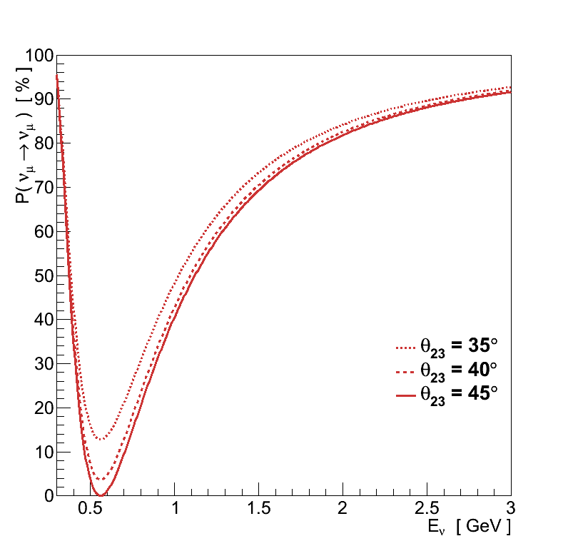
The values of the oscillation parameters then, are determined by measuring the E_ν spectrum for a given flavour before and after traversing the baseline. Any deficits/excesses found are the result of oscillations and the energy, size and shape of those changes can be used to measure the oscillation parameters. We can see this by considering the example of an initially pure ν_μ beam, measured after traversing a baseline of 295 km - approximately equivalent to the T2K experiment (Chapter 5)4Unless specified otherwise, for all the plots in this chapter the oscillation parameters are set to the values in Table 2.1, the initial flux is 100% ν_μ and L = 295 km..

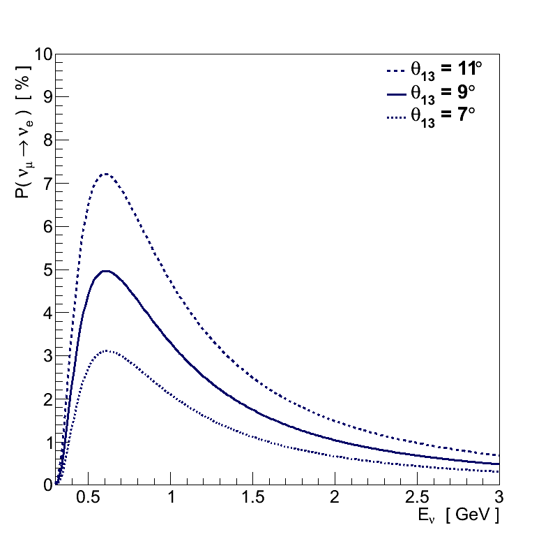
Determination of the mixing angles comes from measurement of the amplitude of oscillations (Figure 2.2). For example, the value of θ₂₃ can be determined from the ν_μ spectrum, where the depth of the minimum resulting from oscillations away from ν_μ indicates the size of θ₂₃. Likewise, measuring the height of the peak in oscillations to ν_e allows the determination of θ₁₃.

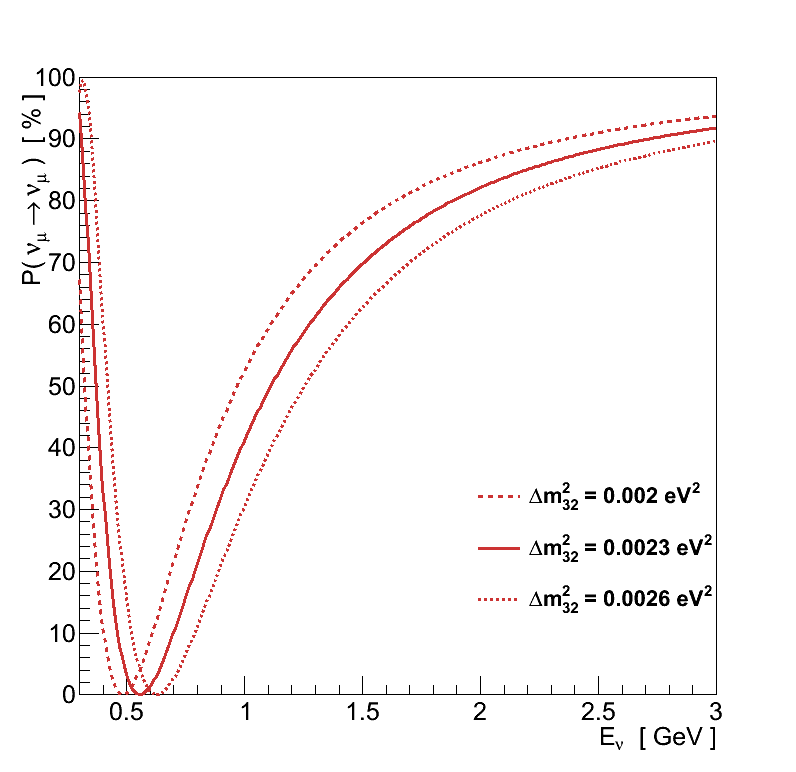
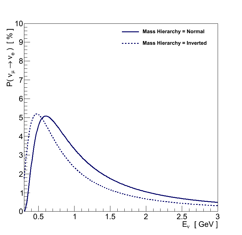
Figure 2.2: (left) The effect of θ₂₃ on P(ν_μ → ν_μ), its value can be determined by measuring the depth of the minimum. (right) The effect of θ₁₃ on P(ν_μ → ν_e), in this case the value can be determined from the height of the peak.

The mass splittings on the other hand affect the energy at which these oscillation features occur (Figure 2.3). The value of Δm²₃₂ can be measured from the E_ν of the minimum in the ν_μ spectrum, and the choice of normal or inverted mass hierarchy results in a shift in the E_ν of the peak in the ν_e spectrum.

Figure 2.3: (left) The effect of Δm²₃₂ on P(ν_μ → ν_μ), the value can be determined by measuring the energy of the minimum. (right) The dominant effect on the ν_e spectrum of changing the mass hierarchy is a shift of the peak's energy.

The long-term goal is to determine whether or not neutrinos violate CP, and perhaps therefore contribute to the matter – anti-matter asymmetry of the Universe. In other words, to measure the value of δ_cp.

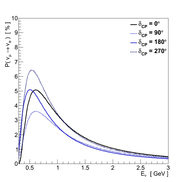
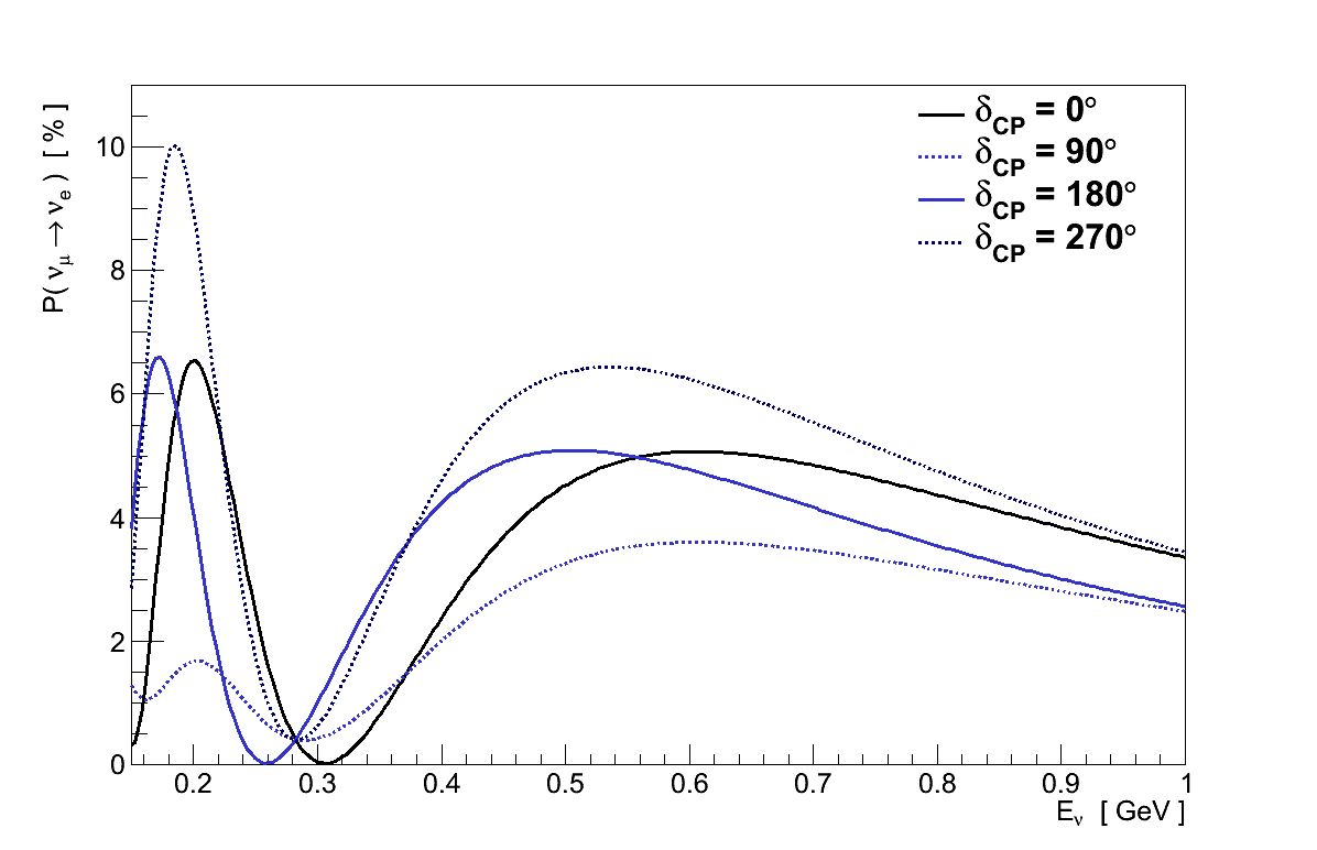
While the other oscillation parameters tend to affect one or other of the amplitude or energy of oscillations, δ_cp affects both (Figure 2.4). As the value of δ_cp is rotated, the position of the ν_e peak varies both in height and energy, traversing a circular path which reaches extremes in amplitude at δ_cp = 90/270 ° and energy at δ_cp = 0/180 °. It also affects ν_e and ν_e differently, with ν_e traversing the same circular path but in the opposite direction. Looking at lower E_ν (Figure 2.5), equivalent to higher L/E_ν, there are additional oscillation peaks which are much more strongly affected by the value of δ_cp.

Figure 2.4: The effect of δ_cp on P(ν_μ → ν_e). (left) As you rotate the angle of δ_cp, the position of the peak follows a circular path, changing both its height and energy. (right) The peak for P(ν_μ → ν_e) follows the same circular path, but in the opposite direction.

This leaves three ways through which such an experiment could determine δ_cp: a precise measurement of the position of the first peak in P(ν_μ → ν_e) spectrum, a comparison of that peak in neutrino and anti-neutrinos or, if the experiment is capable of resolving it, measuring the position of the second P(ν_μ → ν_e) peak.

Figure 2.5: The effect of δ_cp on P(ν_μ → ν_e). If an experiment can resolve the second oscillation maximum at lower E_ν, the effects of δ_cp can be much larger.

However, determining the value of δ_cp through any of these methods will be particularly challenging. Because they only interact weakly, experiments cannot observe neutrinos directly. Instead, they only observe them via the secondary particles produced when they interact. In order to determine the proportion of neutrinos of a given flavour, the experiment must measure the number of events in which the corresponding charged lepton is produced, then use knowledge of the probability of that neutrino interacting to infer the number of neutrinos that actually passed through the detector. In order to measure the energy of the neutrino, the experiment must infer it from measurements of the secondary particles produced, and an understanding of how the neutrino's interaction produced these particles.

Not understanding the probability of a given neutrino flavour interacting will lead to incorrectly determining the number of those neutrinos present, and hence the oscillation probability. Not understanding the kinematics of secondary particles produced by a neutrino's interaction, will result in the energy being mis-reconstructed, and hence the neutrino energy spectrum being distorted. So in order to make precise measurements of the oscillation parameters, a precise understanding of neutrino interactions is needed.

This is particularly true for the determination of δ_cp. The variations in the height and position of the ν_e peak resulting from changes in δ_cp could also be attributed to changes in the values of the mixing angles and mass-splittings. And the size of those variations resulting from δ_cp are much smaller in scale than the current precision in those parameters will allow us to resolve. Furthermore, neutrinos and anti-neutrinos have quite different interaction probabilities, and result in a different range of secondary particles.

So our ability to measure δ_cp is limited by the need for precise knowledge of the other oscillation parameters, and of the interactions of neutrinos and anti-neutrinos. The precision of our knowledge of the other oscillation parameters, is also limited by our understanding of neutrino interactions, and how they relate to the energy and number of neutrinos in our experiment.

In order to increase the precision to which we understand neutrino oscillations, measure δ_cp, and perhaps solve the matter – anti-matter asymmetry of the Universe, we must first understand neutrino interactions.

Footnotes

This is unlike the electromagnetic and strong interactions, whose interaction states are mass eigenstates.
Assuming plane-wavefunctions gives the same results as a more complete treatments in all but extreme cases [5].
There are options for creating mono-energetic neutrinos but none of them are practical. Pion decay at rest would provide a mono-energetic ν_μ source, but their ∼30 MeV energy would be too low for ν_μ CC interactions. Alternatively, Z⁰ decay at rest would make an interesting neutrino source. Around 20% would decay to give an even mix of all six neutrinos and anti-neutrinos at 45.6 GeV. However the oscillation baseline required for such a high energy would be difficult, and the problems in making a high-flux source from stationary Z⁰s are many and large.
Unless specified otherwise, for all the plots in this chapter the oscillation parameters are set to the values in Table 2.1, the initial flux is 100% ν_μ and L = 295 km.