6. A Search for Coherent Pion Production at T2K
In Chapter 4 it was discussed how searches for CC coherent pion production at Eν < 2 GeV have found no evidence for its existence. This is in conflict with the predictions of the established model and additional experimental data is required to resolve the situation. The T2K experiment described in Chapter 5 provides an excellent environment in which to study neutrino interactions at a mean νμ energy of 0.856 GeV, using its near detector ND280. The opportunity was therefore taken to conduct a νμ CC coherent pion production analysis of the ND280 data.
Since there is no experimental evidence that the interaction even exists at these energies, it was decided that the analysis should be conducted as a search, rather than a measurement. The approach was to make a selection of events which should contain any coherent pion interactions which occur, and the events selected in data can then be compared with the non-coherent background predicted by simulation. Any significant excess of events over the background prediction would then indicate that coherent pion production is occurring at an observable rate.
It is always good practice when making physics selections, wherever possible, to focus on the characteristic properties of the sample you wish to select rather than features of the model used to simulate it. This becomes essential when the signal model is considered unreliable, such as in this case where the existing data and model are in conflict. The defining characteristics of νμ CC coherent pion production are:
- Production of exactly one μ- accompanied by one π+
- No fragmentation of the target nucleus
- Low transfer of momentum to the target nucleus, resulting in:
- Little nuclear recoil
- Angles of μ- and π+ with respect to the incoming neutrino are peaked in the forward direction
It is events which match this description, that the analysis must select. This will also improve the reproducibility of the selection by those outside of T2K. If the results of the analysis are to benefit the understanding of coherent pion production, other experiments must be able to perform comparable selections, and theorists must be able to compare them to their predictions.
6.1. Overview
The FGD 1 sub-detector was chosen as the interaction target. It is dense enough to offer a sufficiently high interaction rate, but not so dense as to prevent the majority of π+ from escaping into TPC 2 downstream. It also provides an active volume for better resolving additional activity at the interaction vertex to reject backgrounds. Approximately 0.8 % of the CC νμ interactions in the FGD 1 fiducial volume are predicted to be coherent pion production (using the default Rein-Sehgal model in GENIE).
The first step is the selection of CC νμ interactions, by finding events with a μ- originating from FGD 1. To do this the analysis follows the ND280 νμ Inclusive selection [1] [2], an approved selection used extensively within T2K [3] (Section 6.3). Basing the analysis on this selection gives it a well validated foundation, and improves compatibility with other studies, such as those relating to systematic uncertainties.
The second step is the selection of those CC νμ interactions which also contain a single π+, for which a custom selection was developed (Section 6.4). Finally two cuts are made on the net transverse momentum (Section 6.6) and vertex activity (Section 6.7) in order to reject backgrounds and focus on a more coherent-like sample.
The search for evidence of CC coherent pion production is then performed by looking for an excess over background in the |t| distribution of selected events which, as discussed in Chapter 4, is the characteristic distribution where coherent signals are found.
6.2. Implementation Details
The analysis was implemented in dAnalysis: a self-authored framework, designed for ND280 analyses and written in python. Its interface design focused on simplicity for the user, creating an accessible framework which has been easily utilised by multiple undergraduate project students, and allows rapid prototyping of initial studies. However it also supports more complex requirements and is highly flexible, and is therefore also capable of full analyses, such as this one. The primary drawback of the framework is performance due to being written in a very high-level language. This makes the processing of large numbers of files time consuming. Fortunately, this was only a relevant concern for the initial “skimming” of the full simulated data-set down to a manageable size - a task performed only twice in the development of the analysis.
The data and simulation used come from the official ND280 processing referred to as “production 5”, which at the time of writing is that currently recommended by the ND280 Computing group. The data in this production suitable for analysis is from T2K Runs 1a, 2b, 2c, 3b, and 3c, and was processed through ND280 software version 10.11.21. The quantity of data from each of these runs is measured in terms of protons-on-target (POT), the quantity of protons delivered by the T2K beam onto the target, and is shown in Table 6.1.
| T2K Run | POT Analysed (1020) |
|---|---|
| 1a | 0.29 |
| 2a | 0.13 |
| 2b | 0.65 |
| 3b | 0.21 |
| 3c | 1.35 |
| Total | 2.64 |
The simulation was produced using the neutrino flux prediction from JNUBEAM version 11a (which provided three separate fluxes based on the conditions during T2K Runs 1, 2, and 3), interactions from GENIE version 2.6.6, and ND280 software version 10.11.17. The interactions in this simulation then had three corrections applied:
-
Flux correction
The neutrino flux was updated to JNUBEAM version 11b, which was tuned based on the beam conditions recorded during data running. This is done by taking four histograms of neutrino energy, one for each neutrino flavour, calculating the ratio between the JNUBEAM 11a and 11b predictions for each bin, and weighting every simulated interaction according to the applicable ratio. For νμ interactions these weights range in value from 0.87 to 1.43. -
GENIE coherent pion correction
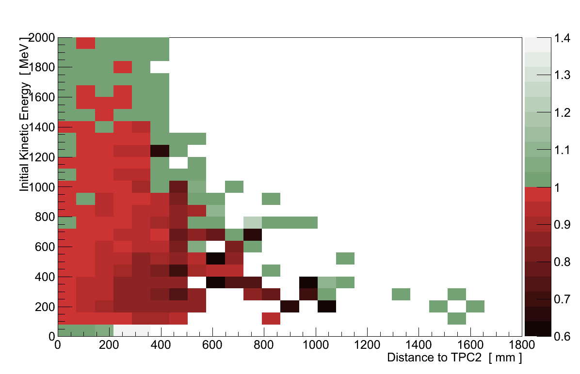
For νμ CC coherent pion interactions in FGD 1 a correction is applied to compensate for a bug in the Rein-Sehgal coherent pion production model implemented in versions of GENIE ≤ 2.8.0 (there was a bug in the interpolation of the pion-nucleon scattering cross-sections, see Figure 6.1). Samples of νμ CC coherent pion interactions were generated on 12C at 100 MeV increments in neutrino energy between 400 and 2000 MeV - both with and without the bug included - each containing 106 events. For each of these samples, a 2D histogram of pion momentum verses angle was made, and the ratio between fixed and unfixed versions is taken to give a weight by which the interactions from simulation are corrected. Typical weights are found within ±30 %.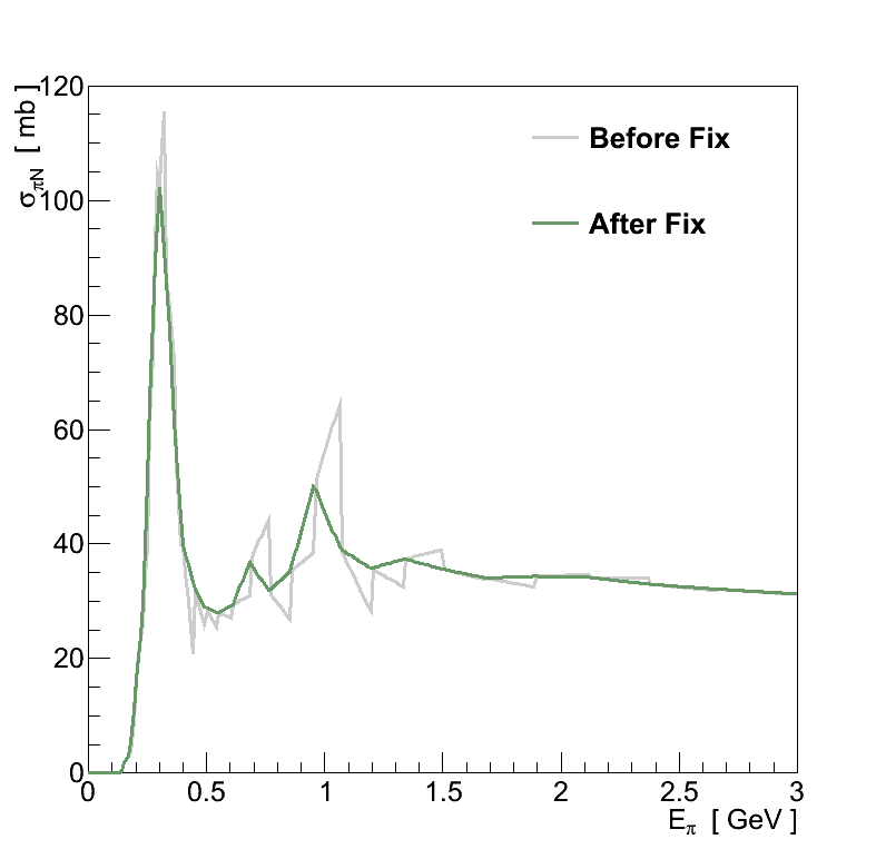
Figure 6.1: Cause and effect of the bug in GENIE's Rein-Sehgal coherent pion production model. (left) The total pion-nucleon scattering cross-section. The inelastic cross-section contains an identical bug. (right) The effect on the pion momentum spectrum for νμ CC coherent pion production on 12C at Eν = 1.0 GeV. -
Momentum resolution correction
The last correction applied to the simulation compensates for the observation that the reconstructed momentum resolutions in data and simulation do not match. Defining pB as the momentum perpendicular to the magnetic field, the resolution on 1/pB was found to be 32 ± 10 % wider in data [4]. Following the prescription in [4], this is accounted for by taking the initial reconstructed 1/pB of selected tracks in simulation and pushing them 32 % further away from their true value such that:(6.1)The reconstructed momentum of the track is then re-calculated from the corrected value of 1/pB. The uncertainty on the resolution difference will appear as a systematic uncertainty in Section 6.10.3.1.
The analysis is also applied to the predictions from two other simulations. Although its coherent pion production model is more dated than that in GENIE, analysing T2K's other interaction simulation, NEUT, provides both an alternative set of background models and a useful reference for those T2K analysers who use NEUT as their primary simulation. NEUT was also the simulation used in the K2K and SciBooNE analyses. The files from production 5 were made with NEUT version 5.1.4.2, to which the same flux and momentum resolution corrections are applied as for Genie.
Additionally the Alvarez-Ruso coherent pion production model which was implemented in GENIE (Section 4.3) allows an assessment of how the signal selection efficiency might by impacted in an alternative model. A sample of 5654 Alvarez-Ruso νμ CC coherent pion events was generated in the FGD 1 fiducial volume and processed through the ND280 software used for production 5. This was merged with the standard production 5 GENIE sample with all Rein-Sehgal coherent events stripped out. The Alvarez-Ruso events were weighted such that the ratio of total Alvarez-Ruso events to total Rein-Sehgal events, was the same as the ratio of their flux-averaged cross-sections, i.e.:
This ensures that the number of events from the Alvarez-Ruso model is normalised appropriately for the analysis, based on the ND280 flux and the model's cross-section.
In this chapter, unless otherwise specified:
- The “signal” is νμ-induced CC coherent pion production inside the fiducial volume defined in Section 6.3
- Data is from T2K Runs 1a, 2b, 2c, 3b and 3c combined
- Simulation is from T2K Runs 1a, 2b, 2c, 3b and 3c combined, scaled run-by-run to match the POT recorded in data, produced with GENIE and with the corrections detailed above applied
- Plots show both data and simulation as histograms, simulation represented by solid boxes, and data by crosses (the horizontal width indicating the extent of the bin, and the vertical height a Gaussian statistical uncertainty)
- The abbreviation OOFV refers to interactions which occurred outside of the fiducial volume
6.3. The νμ Inclusive Selection
The νμ Inclusive selection was developed within the ND280 νμ analysis group and was re-implemented for this analysis based on its description in two internal technical notes [1] [2]. However the selection was originally developed for production 4, and the benefits from reconstruction and calibration improvements in production 5 have resulted in a few notable differences between this implementation and the original:
- The momentum for tracks is taken from the global ND280 reconstruction instead of the TPC reconstruction.
- The dE/dx values provided by the TPC reconstruction no longer require correcting.
- The fiducial volume is modified from that in the original (see below).
The νμ Inclusive selection is made by passing through the following steps:
-
Require good data quality
For each beam spill the T2K Beam Group determine whether or not the spill was of good quality by requiring stable operation of the beam magnets and horns, and the signal in the muon monitors being in the correct direction and within a target intensity. Likewise the ND280 Data Quality group assess whether the ND280 was operating correctly by checking the operation of all five sub-detector systems and the magnet. For data from a spill to be included in the analysis, both of these groups must have approved it for use. -
Separate trigger into bunches
The ND280 detector is triggered once per beam spill so the tracks must be separated out into the bunches they belong to (Figure 6.2). A track is deemed to belong to a bunch if its start time lies within 60 ns of the mean bunch time (in data bunches are approximately 15 ns wide separated by around 550 ns). From here on, the term “event” will be taken to mean the contents of a single bunch. -
Select a candidate muon track.
The signature feature of a νμ CC interaction is the presence of a muon - a negatively charged particle which will likely be highly penetrating and leave a long, clean track. So the first selection requirement is to search the event for reconstructed tracks which:- Are negatively charged
-
Include a “good” component in TPC 2
A “good” TPC component is one formed of hits on 18 or more of the micromegas’ readout columns. Because the TPC reconstruction is based on first clustering hits vertically, this ensures that the track is of sufficiently high quality that the charge and PID information are reliable. -
Start within the FGD 1 fiducial volume
The original νμ Inclusive selection defined the fiducial volume to exclude the first two upstream layers, and the outer-most five bars at either end of each subsequent layer (Figure 6.2). In this analysis the fiducial volume was modified to also exclude the final two downstream layers, which was necessary to ensure the vertex activity could be measured consistently (Section 6.7).
If no reconstructed tracks are found to meet these requirements the event is rejected. If one or more tracks is found the one with the highest momentum is chosen. This reconstructed track is referred to as the “muon candidate”.
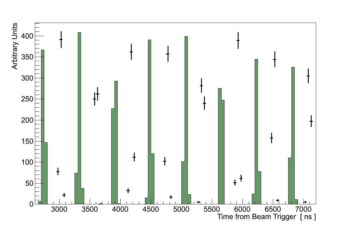
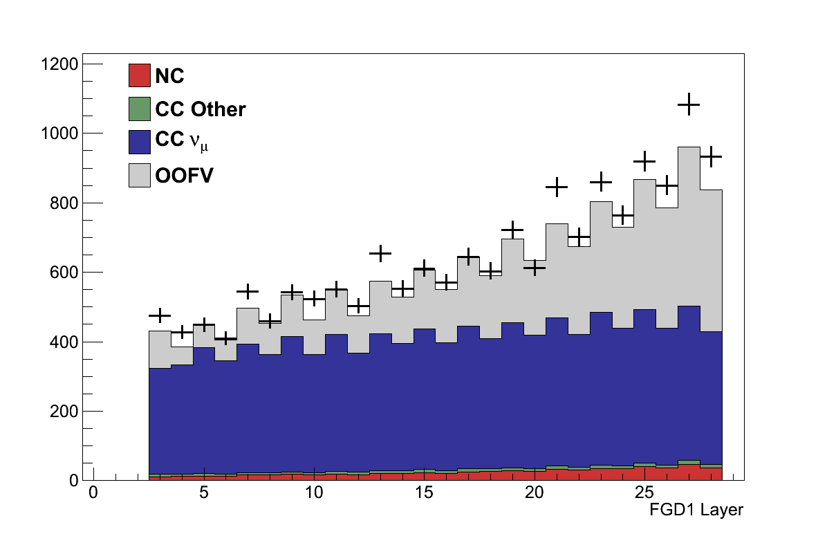
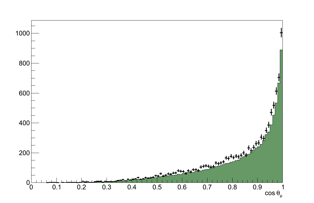
Figure 6.2: (Left) The time relative to the beam trigger of selected muon candidates. The bunches in each T2K run and simulation occur at different times, so for the sake of clarity only data from T2K Run 2b is shown. (Right) The FGD 1 layer in which the starting position of selected muon candidates is found. The simulation is broken down by the true interaction. -
Veto backwards-going tracks
If the end position of the muon candidate is upstream of its start position then the event is rejected. This cut was added in response to the observation that most negative tracks which were reconstructed as backwards-going were in fact forward-going positive tracks1The reconstruction determines the direction of a track based on which alternative provides a better fit for the Kalman filter it uses.. Due to improvements in the reconstruction this is no longer necessary, however the cut has been left in the analysis for consistency with the original νμ Inclusive selection. It removes only 0.2 % of tracks which, in any case, are likely to be mis-reconstructed (Figure 6.3).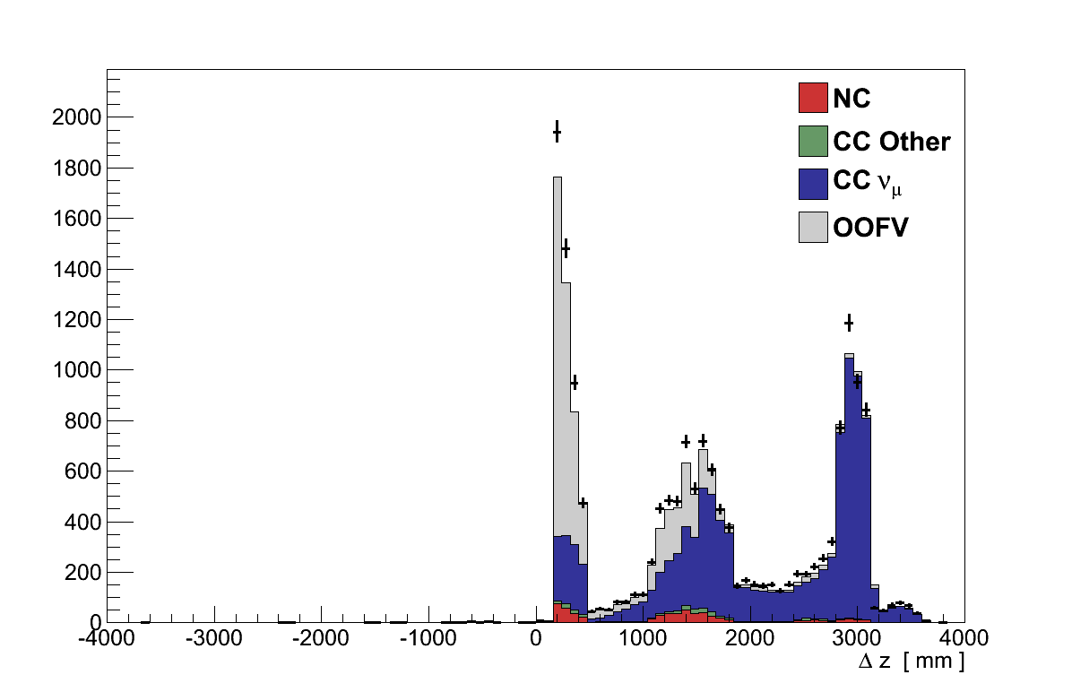
Figure 6.3: The difference in z-position of the front and back of the muon candidate track. The first peak contains low-momentum tracks curving quickly out of TPC 2, the central peak comes from tracks stopping in FGD 2, and the last peak stopping in the Ds ECal. Events with Δz < 0.0 are rejected. -
Veto tracks coming from upstream
This cut attempts to remove events which originated further upstream than FGD 1 but resulted in a separate reconstructed track emerging from FGD 1. To do this, all the other tracks in the event (same beam-bunch as the muon candidate) that have a good TPC component are selected. Then the highest momentum track in this selection is chosen. If the start position of that track is >150 mm upstream of the muon candidate's start position, then the event is rejected (Figure 6.4).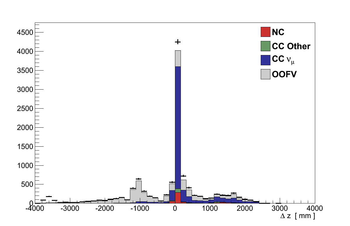
Figure 6.4: The difference in z-position of the front of the muon candidate track and the front of the second track. If Δz < -150 mm the event is rejected. The un-simulated bump in data at Δz ≈ -3600 mm is likely due to muons from interactions upstream of the detector, known as “sand muons”, which are not included in the standard simulation. -
Require muon candidate track to be muon-like
As discussed in Section 5.4.3, the TPCs provide discriminating variables for particle identification (PID). First, the truncated mean of the energy deposited in the TPC is taken to be the measured dE/dx of the track. Pull variables Pi are then formed by comparing this to the dE/dx expected at the track’s momentum for four particle hypotheses, i (proton, charged pion, muon and electron). Finally, likelihoods formed from these pulls are combined into discriminating variables Xi for each particle hypothesis:(6.3)which give values ranging from 0 (indicating that particle hypothesis is worse than the others) to 1 (indicating that particle hypothesis is better than the others). In addition, for tracks with momentum < 500 MeV an additional PID discriminator is calculated:
(6.4)This is to separate electrons from minimally ionising particles (MIPs, i.e. muons and pions) whose dE/dx profiles overlap at low-momenta (see Figure 5.15).
Cuts are then applied using these discriminators calculated for the muon candidate. For events where the candidate has momentum ≥ 500 MeV the event is rejected if Xμ ≤ 0.05. For events where the candidate has momentum < 500 MeV the event is rejected if Xμ ≤ 0.05 or YMIP ≤ 0.8 (Figure 6.5).

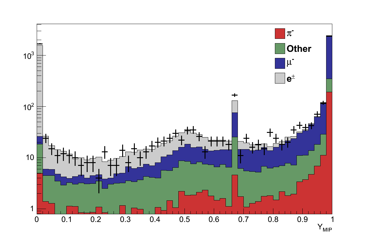
Figure 6.5: (left) Plot of Xμ for all muon candidates. (right) Plot of YMIP for muon candidates with momentum < 500 MeV, shown on a log scale because the distribution is dominated by the spikes at 0 and 1.
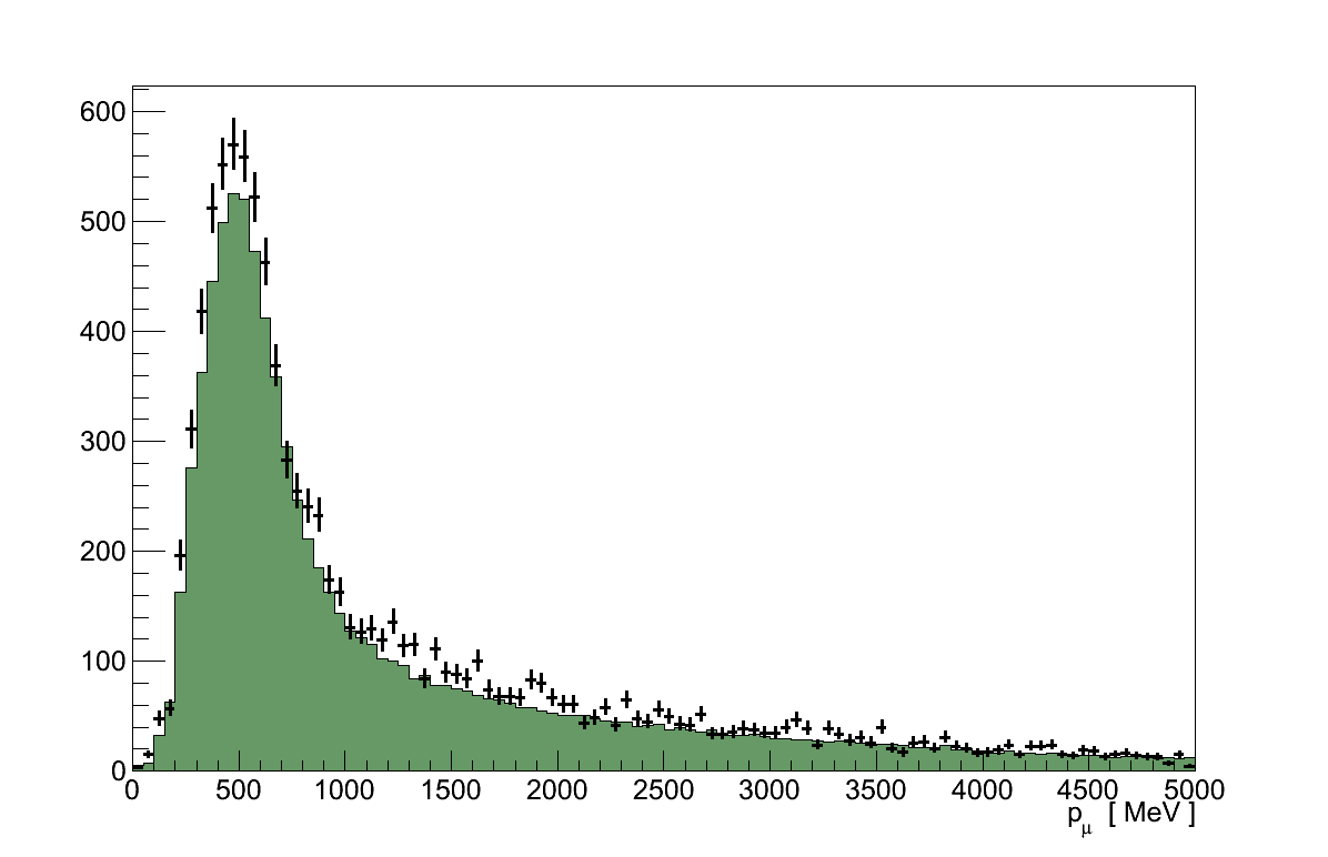
The events which pass these requirements are referred to as the ND280 νμ Inclusive Selection, and in data it contains 10318 tracks. According to the simulation, in which the selection contains 9005 tracks, this is a 90 % pure sample of muons. Aside from the overall normalisation difference, the momentum and angular distributions are well described by the simulation (Figure 6.6).
6.4. The Coherent Initial Selection
After selecting CC νμ events, the selection now needs to be refined to those which match the appearance of coherent pion production. Specifically that means a μ- and π+ originating within FGD 1, travelling downstream, and unaccompanied by other particles. This is done by applying the following requirements to each event:
-
Veto excessive tracks in FGD 1
True coherent interactions should produce exactly one muon and one pion, so the presence of any additional tracks in the target detector is a strong indicator that this is not a coherent interaction. Therefore, events in which FGD 1 contains more than two reconstructed objects are rejected (Figure 6.7).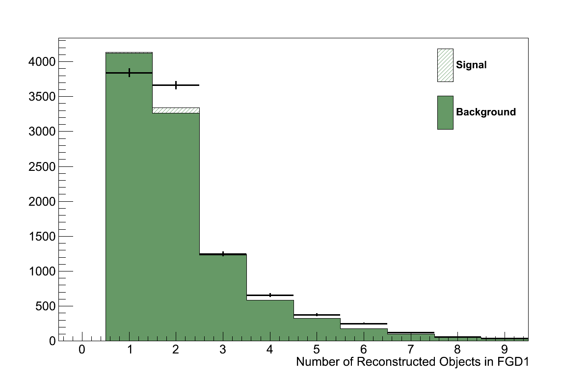
Figure 6.7: The number of reconstructed objects in FGD 1 -
Select a candidate pion track
In addition to the muon, for which a candidate track has already been selected, coherent interactions should also produce a π+. So the event is searched for tracks which:- Are positively charged
-
Include a “good” component in TPC 2
Where “good” is defined the same as for the muon candidate. -
Are pion-like
The track is rejected if Xπ ≤ 0.05 -
Are not proton-like
As can be seen in Figure 6.8, the largest background when selecting secondary positive tracks is protons, so this is mitigated by rejecting tracks where Xp ≥ 0.5
Note that there is no requirement that the tracks include a component in FGD 1. Because it is a challenging task for the FGD reconstruction to separate two close, parallel tracks (such as a forward-going muon-pion pair), no requirement is placed on the track being reconstructed in FGD 1 or being associated with the muon candidate's vertex.
If no tracks are found which meet these criteria the event is rejected. If more than one track is found the event is also rejected, on the grounds that coherent events should not contain multiple tracks. If exactly one track is found, that track is referred to as the “pion candidate”.
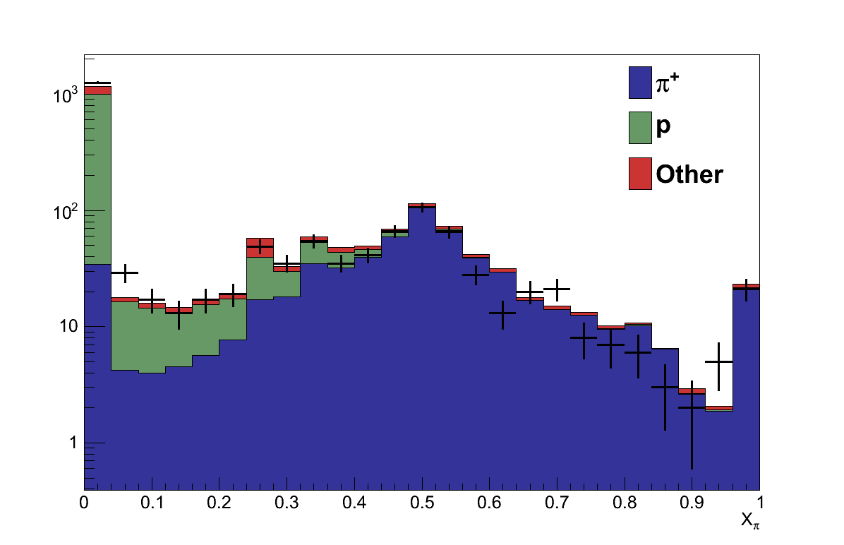
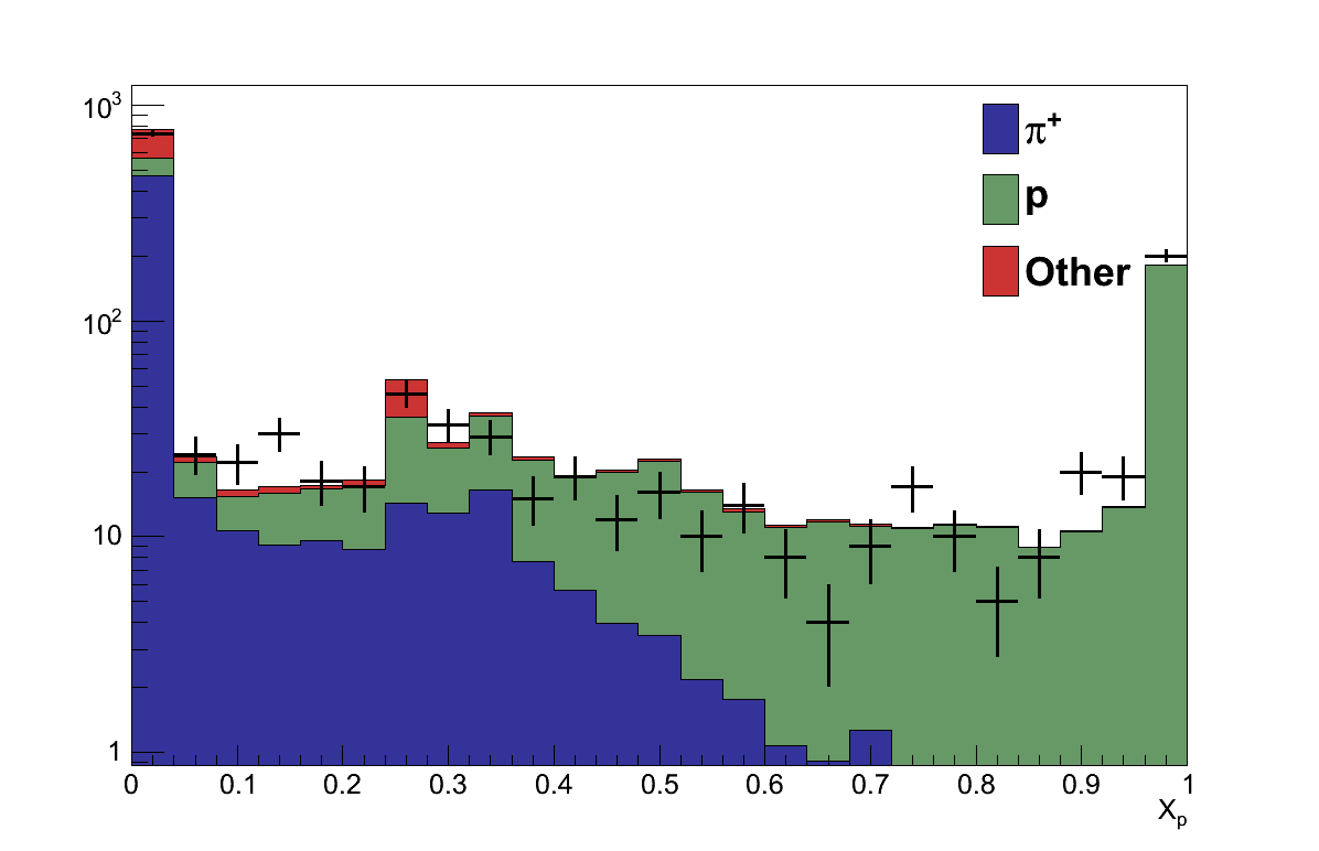
Figure 6.8: (left) Plot of Xπ for all potential pion candidates. Candidates with Xπ ≤ 0.05 are rejected. (right) Plot of Xp for all potential pion candidates. Candidates with Xp ≥ 0.5 are rejected. Both are shown on log scales because the distributions are dominated by the spikes at 0.
The events which pass these requirements form the coherent initial selection, of which there are 620 in data. This compares with the prediction from simulation of 704 events which, for the default Rein-Sehgal coherent model, is expected to include 42 % of the true coherent interactions which took place (Table 6.2).
Of the signal events lost, 38 % were discarded by the νμ Inclusive Selection, predominantly as a result of failing to find a good negative track in both FGD 1 and TPC 2. The remaining 62 % lost were discarded by the coherent pion selection. The largest single drop comes in failing to find a good positive track in TPC 2 - a result of pions being absorbed in FGD 1 or escaping out of the sides of the detector. In future productions, as the ND280 reconstruction improves, it may become possible to recover some of the lost efficiency by selecting tracks which are contained within FGD 1, or escape into the surrounding ECals.
| Step | Data | Simulation | |||
|---|---|---|---|---|---|
| Total | Signal | Efficiency | Purity | ||
| νμ Inclusive selection | 10303 | 10016 | 96 | 78 % | 1.0 % |
| FGD 1 veto | 5275 | 4821 | 83 | 67 % | 1.7 % |
| Positive track in TPC 2 | 627 | 711 | 52 | 43 % | 7.3 % |
| Pion PID | 620 | 704 | 52 | 42 % | 7.4 % |
Thus far the focus of the selection has been on finding signal events, those containing just a muon and a pion, rather than removing any backgrounds. As can be seen in Table 6.3, the primary cause of failure of that goal is in mis-identification of the candidate pion track. The biggest single contamination (Table 6.4) is of protons which can be seen in Figure 6.9 to be mostly found at p > 1000 MeV where the TPC PID is less able to distinguish protons from pions (Figure 5.15). Likewise, contaminations of electrons and positrons can mostly be found at p < 300 MeV where again the TPC PID curves overlap.
| Good Muon | Bad Muon | |
|---|---|---|
| Good Pion | 71% | 5% |
| Bad Pion | 19% | 5% |
| Particle | π+ | p | μ+ | e- | e+ | K+ | Other |
|---|---|---|---|---|---|---|---|
| Fraction | 78 % | 14 % | 4 % | 1 % | 1 % | 1 % | < 1 % |
| Final State Particle Topology | Fraction of Events |
|---|---|
| Muon + Pion | 32 % |
| Muon + Proton + Pion | 23 % |
| Muon + Pion + X | 19 % |
| Muon + Proton | 8 % |
| Muon + X (no pion) | 7 % |
| NC + Pion + X | 4 % |
| OOFV | 4 % |
| Anti-Muon + Pion + X | 1 % |
| Muon + Nothing | 1 % |
| Other | < 1 % |
With a selection of coherent-like events, the next task is to reduce the background contamination. This is achieved by cutting on variables which highlight characteristic features of coherent pion production, and separate it from background interactions.
Two such cuts are applied. First, a cut on the net transverse momentum of the muon-pion system exploits the kinematic requirements on a predominantly two-body interaction. Second, a cut on the amount of energy deposited near the vertex attempts to exclude events which generated additional particles which were un-reconstructed.
6.5. Neutrino Direction Correction
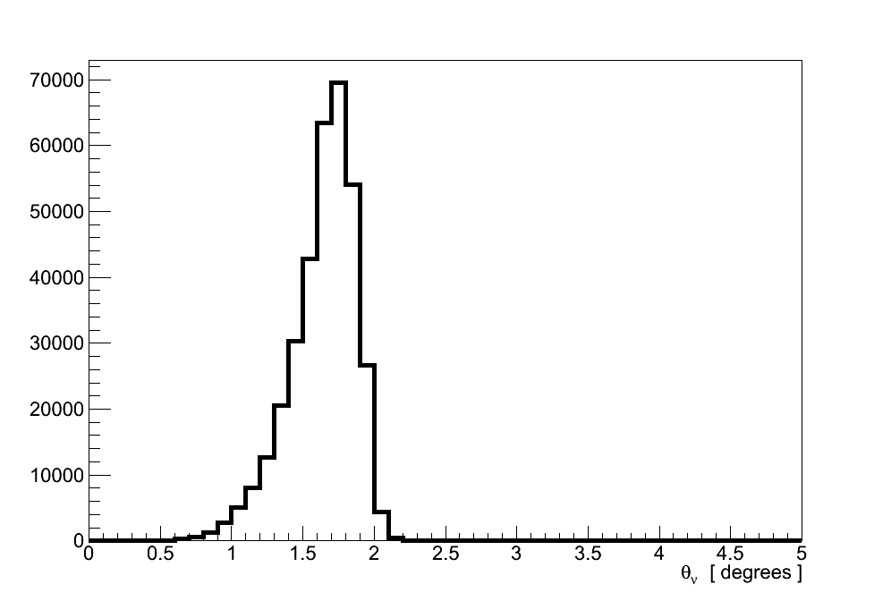
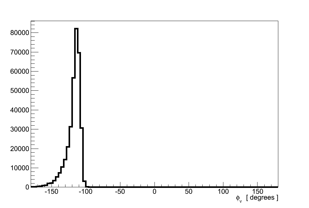
Before proceeding a small correction is made to the track directions output by the ND280 reconstruction, in both data and simulation, to account for the difference between the detector's co-ordinate system and the direction defined by the incoming neutrino. As can be seen in Figure 6.10, neutrinos in the fiducial volume are peaked at an angle of θν ≈ 1.7 ° with respect to the detector's z-axis. In the transverse plane they are found with -180 ° < φν < -100 °: corresponding to travelling upwards and to the right if looking downstream.
On average the final-state particles resulting from a neutrino interaction are produced isotropically in the plane perpendicular to the direction of the incoming neutrino. However the offset described above results in anisotropy when measured in the detector's co-ordinate system. For most measurements this difference is negligible, however it is more significant when dealing with transverse distributions.
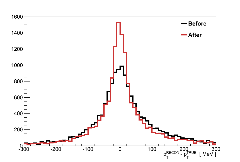
Since this analysis will make a cut on transverse momentum, a correction is made to reduce this effect by rotating the directions/momenta of reconstructed objects to align with the mean neutrino direction. Using a large sample of true CC νμ interactions in the fiducial volume, the mean neutrino direction is calculated as uν = (-0.0127 , -0.0253 , 0.9996), with an angle θu = 1.62 °.
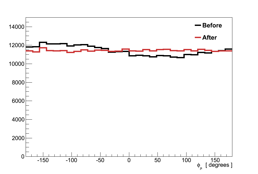
As shown in Figure 6.11, this correction flattens out the anisotropy in the transverse angle of primary muons. More importantly, in Figure 6.12, this correction results in a more accurate measurement of the transverse momentum of the muon-pion system (defined in Section 6.6) for events in the coherent selection, reducing the RMS from 97 to 86 MeV, a roughly 10% improvement.
6.6. Transverse Momentum Cut
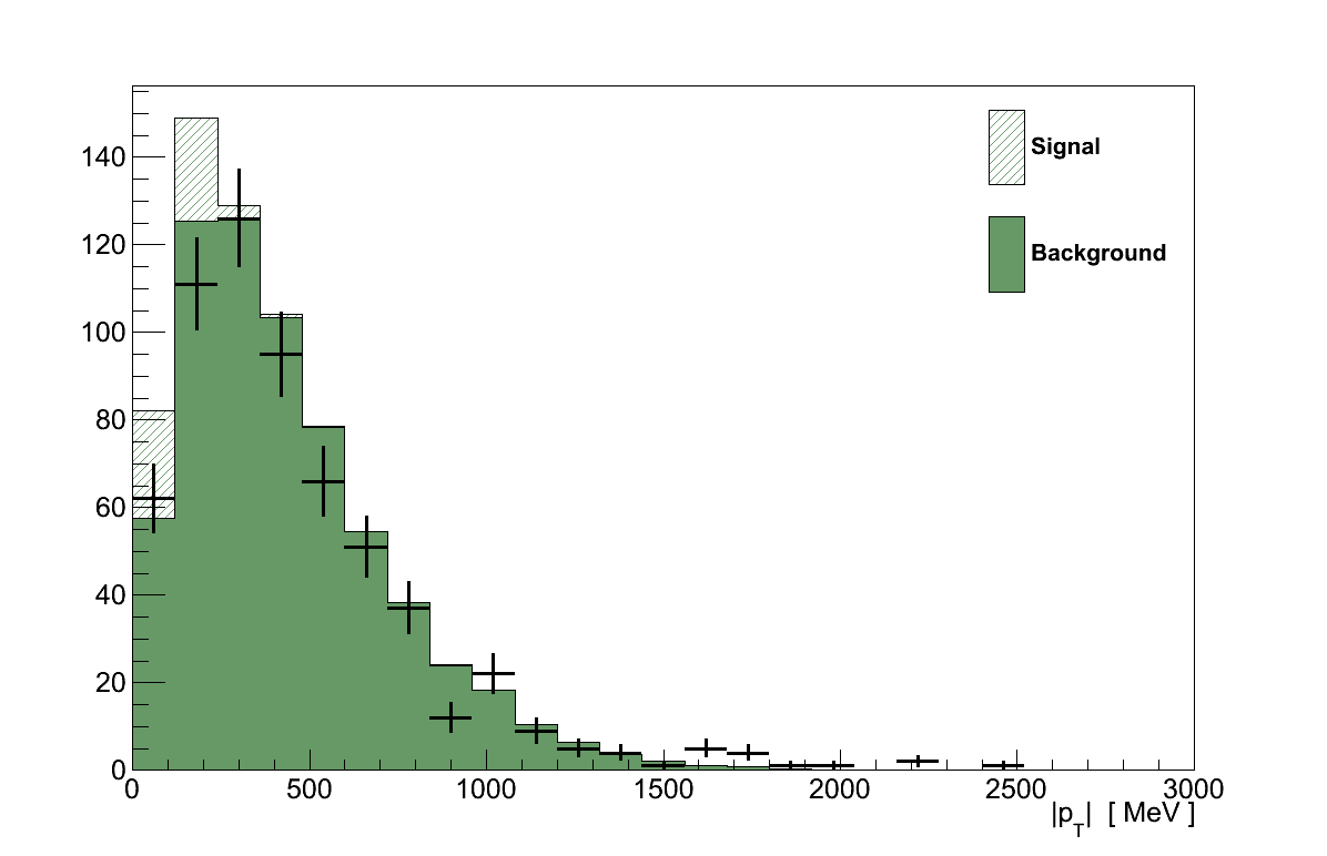
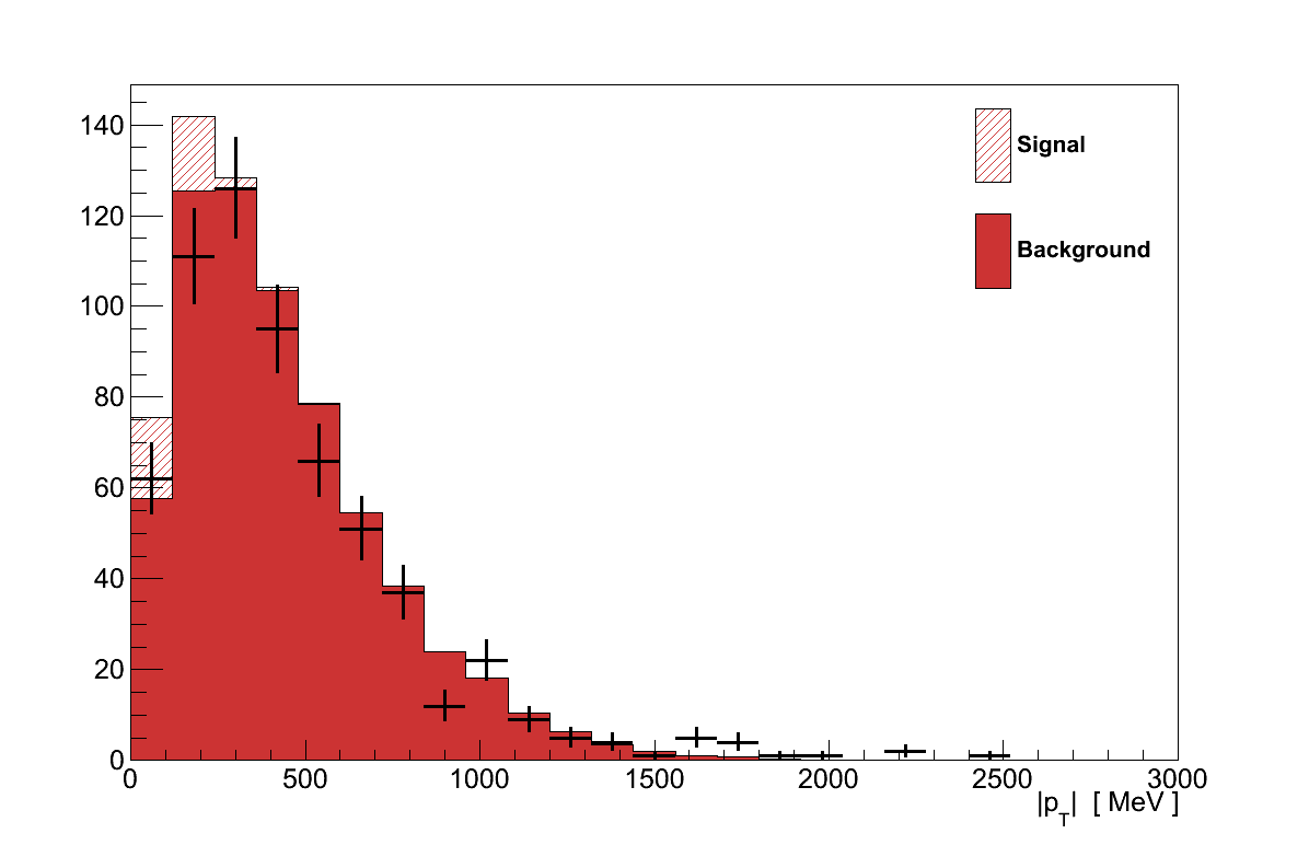
With the coherent selection made the next task is to reduce the amount of background that has come with it. This is done by cutting on two distributions, the first of which is on the total transverse momentum of the muon-pion system, pT.
Under the assumption that the target nucleus with which a neutrino interacts is stationary, conservation of momentum requires that the complete system of final-state particles has no net momentum transverse to the incoming neutrino's direction. Although coherent interactions can transfer some momentum to the nucleus any large transfer would break coherence, so pT tends to be small. Meanwhile background interactions which generated additional, unreconstructed particles can give larger values of pT since the muon and pion no longer represent the complete final-state.
The value of pT is calculated by taking the magnitude of the transverse component, of the vector sum of the muon and pion reconstructed momenta:
As can be seen in Figure 6.13, coherent interactions tend to have low pT while the background distribution extends to higher values. By maximising the product of signal efficiency and purity a cut value of 190 MeV was set, above which events are rejected.
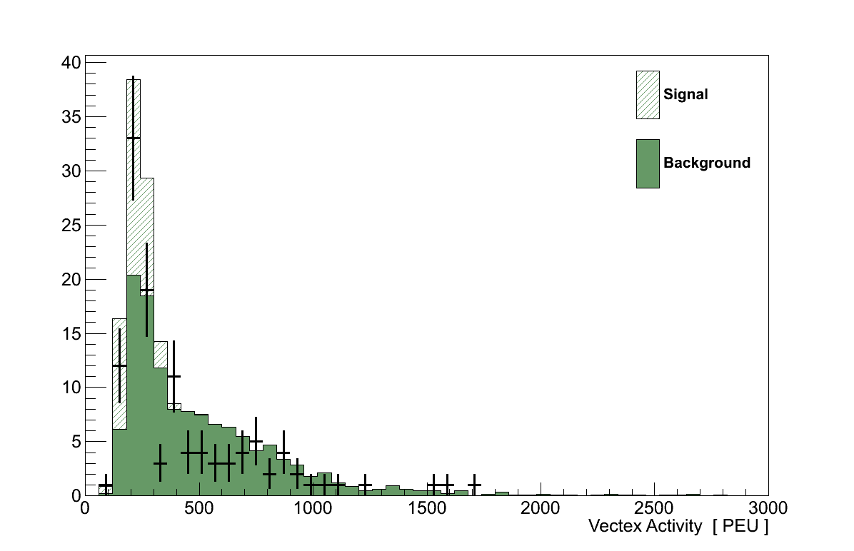
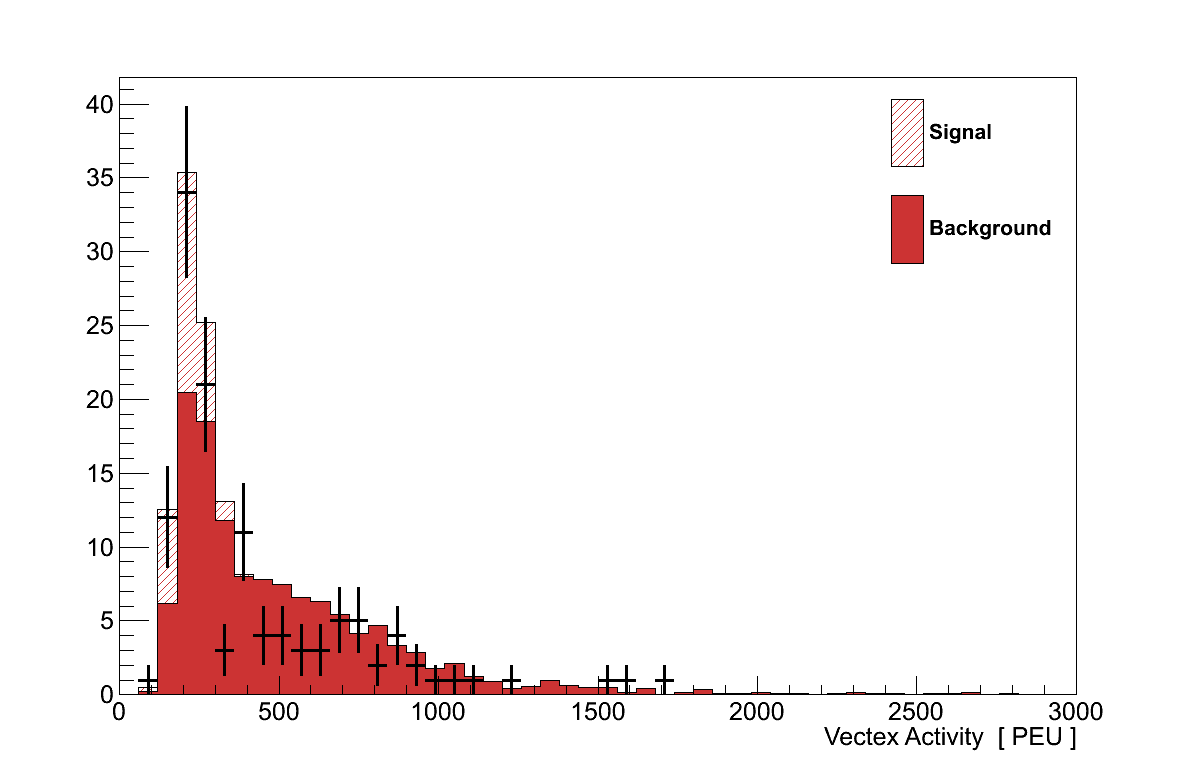
6.7. Vertex Activity Cut
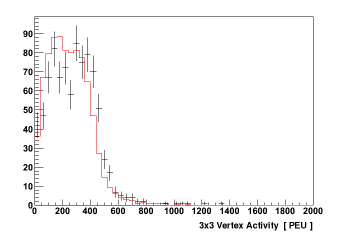
The second cut is made on the “vertex activity” (VA) in FGD 1 - a measure of the energy deposited around the vertex. This includes deposition from particles which produced reconstructed tracks and, crucially, also from short ranged particles which could not be reconstructed. The value of VA therefore is sensitive to the existence of additional final-state particles which exited the nucleus after a neutrino interaction, but did not have enough momentum to travel a sufficient distance in the detector to be reconstructed. Coherent interactions, which generate only a muon and pion, should have low VAs. Background events meanwhile may have generated any number of low momentum protons or pions which, if they exited the nucleus, will have deposited their energy in the surrounding bars and increased the VA.
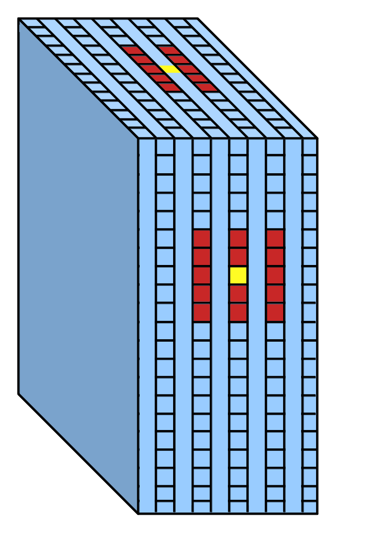
The VA is calculated for every track which starts inside the detector. Its calculation is illustrated by Figure 6.14. The 3D fitted position of the track's start is taken to be the vertex. Then a box is formed centred on the vertex, 5 layers deep and 5 × 5 bars high/wide, and all the bars in that volume are selected. The attenuation-corrected energy deposited in each of these bars is then summed to give the VA at the start of that track. No attempt is made to subtract the contributions from the muon and pion tracks to the energy deposited. Since there are two tracks associated with each event, the muon and pion candidates, the VA for the event is taken from the track with the upstream-most starting position.
The high VA tail generated by background events can be clearly seen in Figure 6.15, with coherent events all found peaked at lower values. By maximising the product of signal efficiency and purity a cut value of 290 PEU was set, above which events are rejected.
6.8. Selection Performance
The events which remain after these cuts are the coherent selection, which comprises 65 events in data. This compares with 81 events in the POT-scaled simulation, 39 of which are coherent signal interactions - an efficiency of 32 % and a purity of 48 % (Table 6.6).
| Step | Data | Simulation | |||
|---|---|---|---|---|---|
| Total | Signal | Efficiency | Purity | ||
| νμ Inclusive selection | 10303 | 10016 | 96 | 78 % | 1.0 % |
| Coherent Initial selection | 620 | 704 | 52 | 42 % | 7.4 % |
| pT cut | 122 | 169 | 43 | 35 % | 25.3 % |
| VA cut | 65 | 81 | 39 | 32 % | 47.8 % |
As can be seen in Table 6.7, 76 % of the interactions selected were ones which included both a muon and pion. Ultimately, if an interaction produces a forward-going muon-pion pair with little or no momentum carried away by other particles, there is no way to separate it from a true coherent event.
Approximately half of the remaining background comes from events containing only a muon and a proton. At high-momentum the dE/dx of protons is similar to that of pions, making it difficult to separate this background out using the TPC PID. In future productions, where the ECal PID information is available, it may be possible to reduce this component. Some of the remaining topologies, such as OOFV or a lone muon, are likely the result of failures in the reconstruction, which again could be reduced by improvements in future versions of the ND280 software.
| Topology | Fraction |
|---|---|
| Muon + Pion | 65 % |
| Muon + Proton | 13 % |
| Muon + Pion + X | 10 % |
| Anti-Muon + Pion + X | 3 % |
| Muon + X (no pion) | 2 % |
| Muon + Nothing | 2 % |
| OOFV | 2 % |
| NC + Pion + X | 2 % |
| Muon + Proton + Pion | 1 % |
| Other | < 1 % |
The interaction modes used by GENIE to generate the simulated events in the coherent selection are listed in Table 6.8. You may recall that the discussion in Chapter 3 concluded that experiments should be concerned with particle topologies, rather than simulator interaction models. However the interaction model used to simulate the background becomes relevant when considering the systematic uncertainties on that background prediction (Section 6.10.2).
| Interaction | Fraction |
|---|---|
| CC νμ Coherent | 48 % |
| CC νμ Resonance | 21 % |
| CC νμ QE | 12 % |
| CC νμ DIS | 12 % |
| CC νμ | 3 % |
| OOFV | 2 % |
| NC | 2 % |
| CC νe / CC νe | < 1 % |
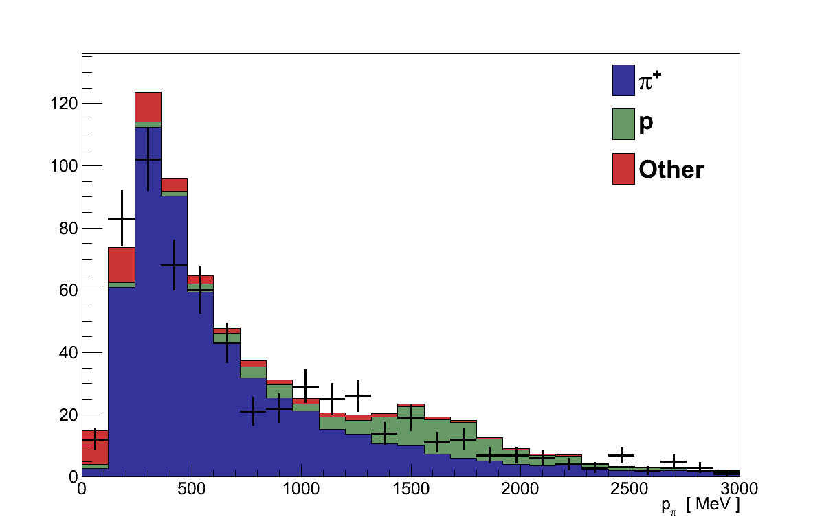
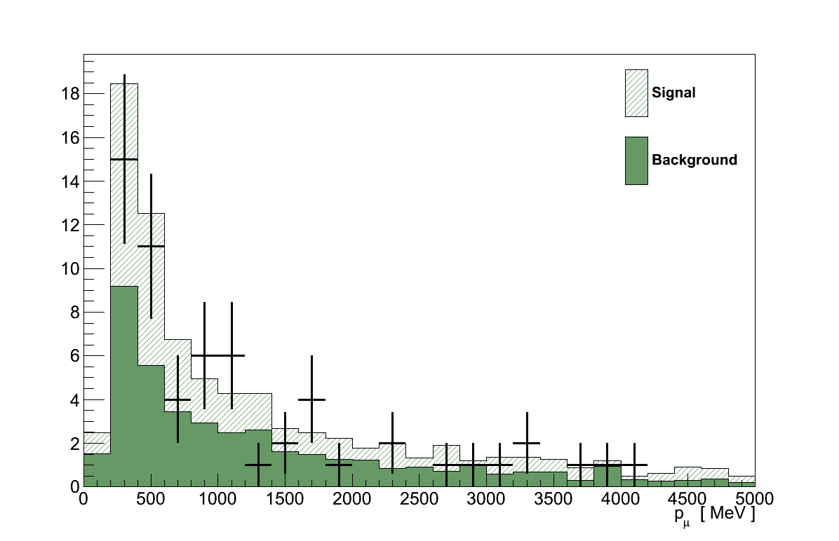
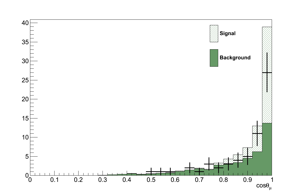
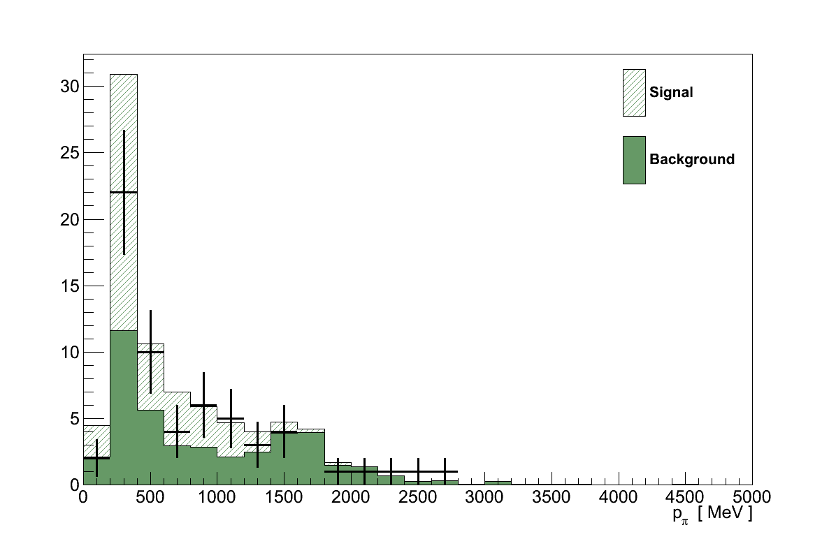
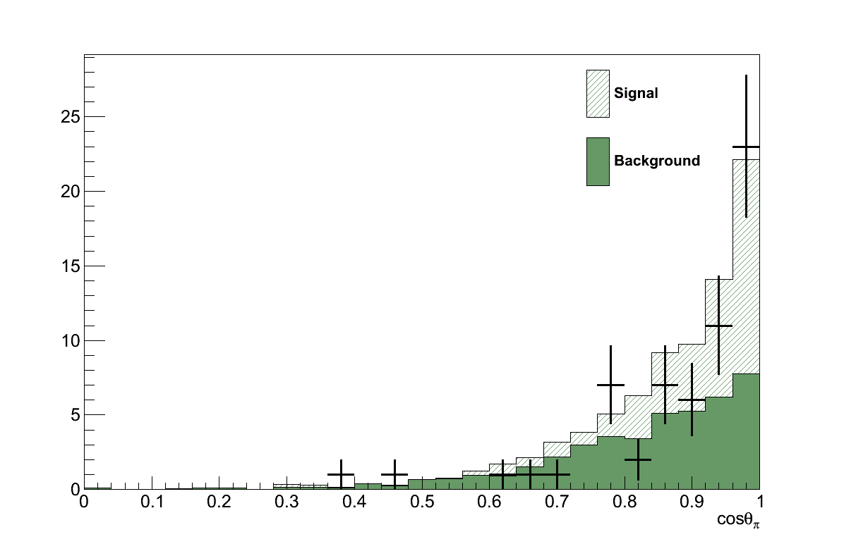
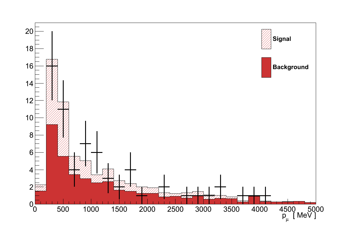
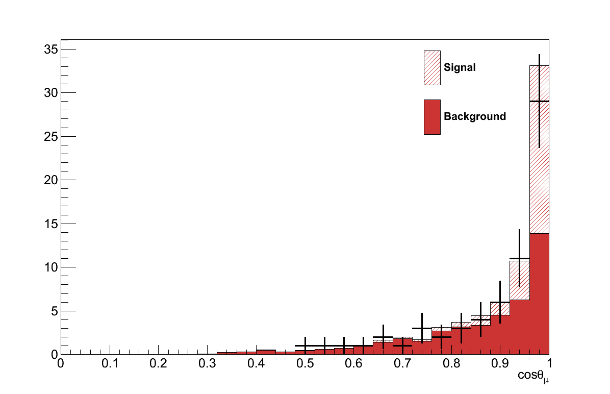
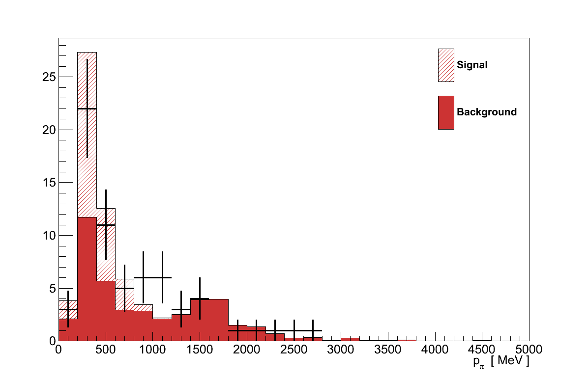
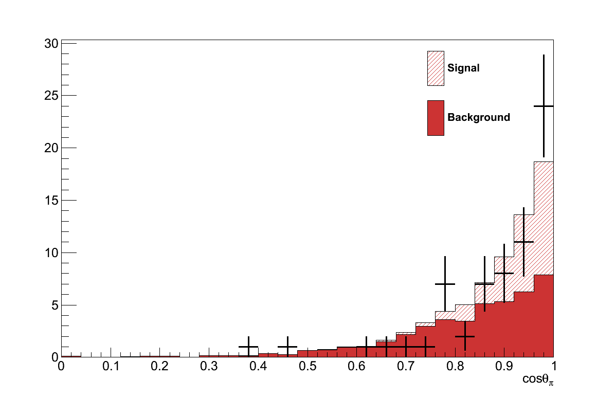
Finally, Figure 6.16 shows the momenta and angles of the muon and pion candidate tracks from the coherent selection. Critically, there are no concerning features in these plots that would suggest the presence of an un-accounted background.
6.9. The Result Calculation Procedure
The goal of this analysis is to conduct a search for coherent pion production, and so far a sample of events which is tuned to select such interactions (if they take place) has been made. If coherent pion production is not taking place, or is doing so at a rate below the resolution of this analysis, the data in this selection should be consistent with the background prediction from simulation. If however there is a signal from coherent pion production, an excess of data above the background prediction could be observed. The remaining task then, is to define a method of assessing whether or not there is an excess of data above the background prediction, and if so how significant that excess is.
As discussed in Chapter 3, there are significant uncertainties surrounding the simulation of our background processes, so the method should attempt to reduce its sensitivity to such uncertainties. It is also important that any excess detected should be consistent with the type of excess expected of a coherent signal - not just a general excess in the number of events selected.
The method chosen was to pick a kinematic distribution in which coherent pion production has a characteristic behaviour. This distribution is then separated into a “signal region”, where coherent events would be expected to appear in addition to some background, and a “control region” which contains only background events. The number of events in the control region can then be used to constrain the expected number of background events in the signal region - removing uncertainties from the absolute normalisation of the background. Using this constrained background prediction, an excess of events can be sought in the signal region.
A distribution which meets these requirements is |t|:
The four-momenta of the muon and pion, Pμ and Pπ, can be determined from the three-momenta measured in the detector, however the neutrino's four-momentum, Pν, must be inferred. By making the assumption that the recoiling nucleus takes only momentum, and no energy, from the interaction - an assumption commonly referred to as the “infinitely heavy nucleus” - the neutrino's four-momentum is taken to be:
which gives all the information required to calculate |t|.
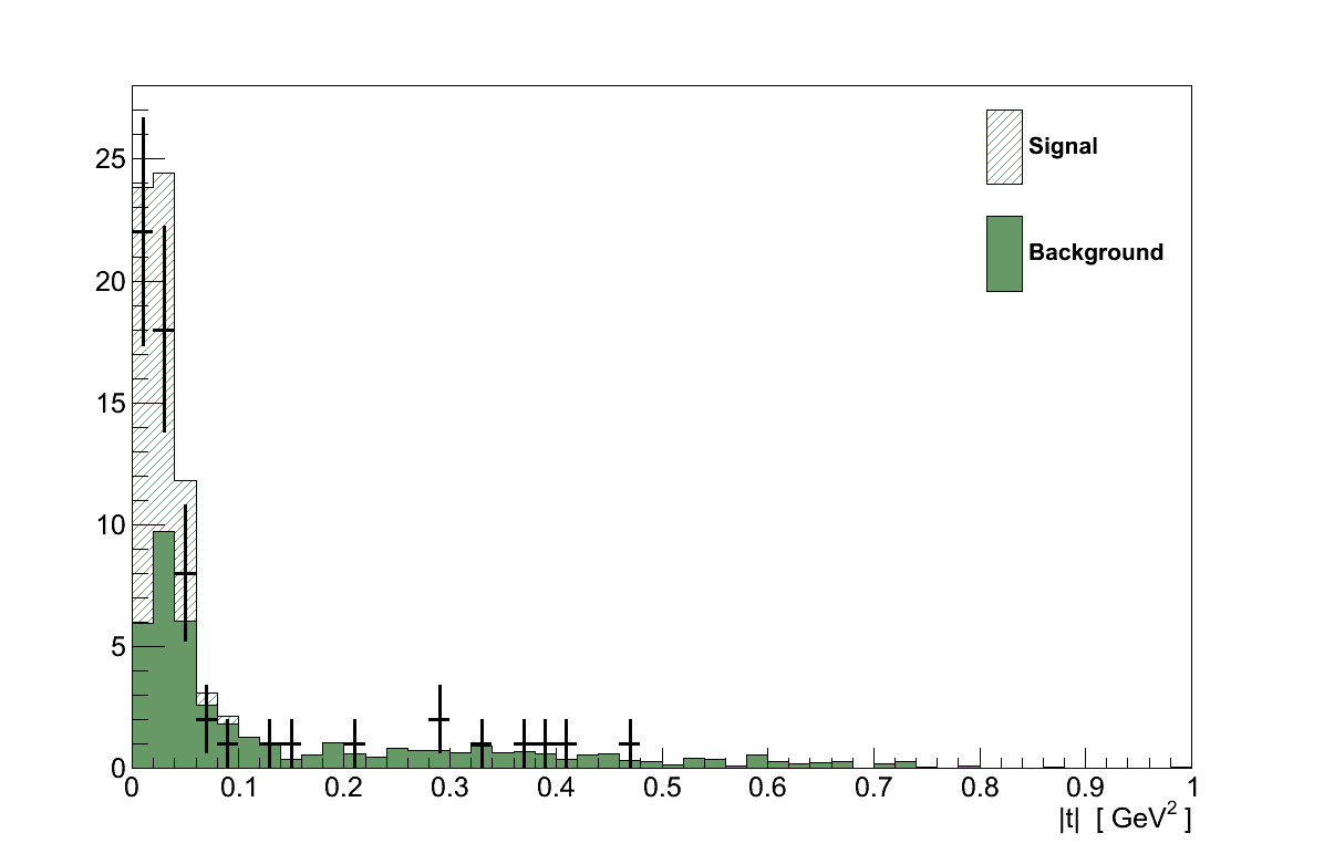
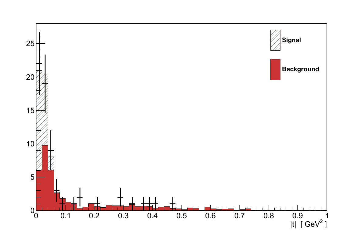
Recalling Chapter 4, |t| is a measure of the momentum transfer to the nucleus, small values of which is a characteristic feature of coherent interactions as can be seen in Figure 6.17. This makes |t| an ideal match to the requirements set out above.
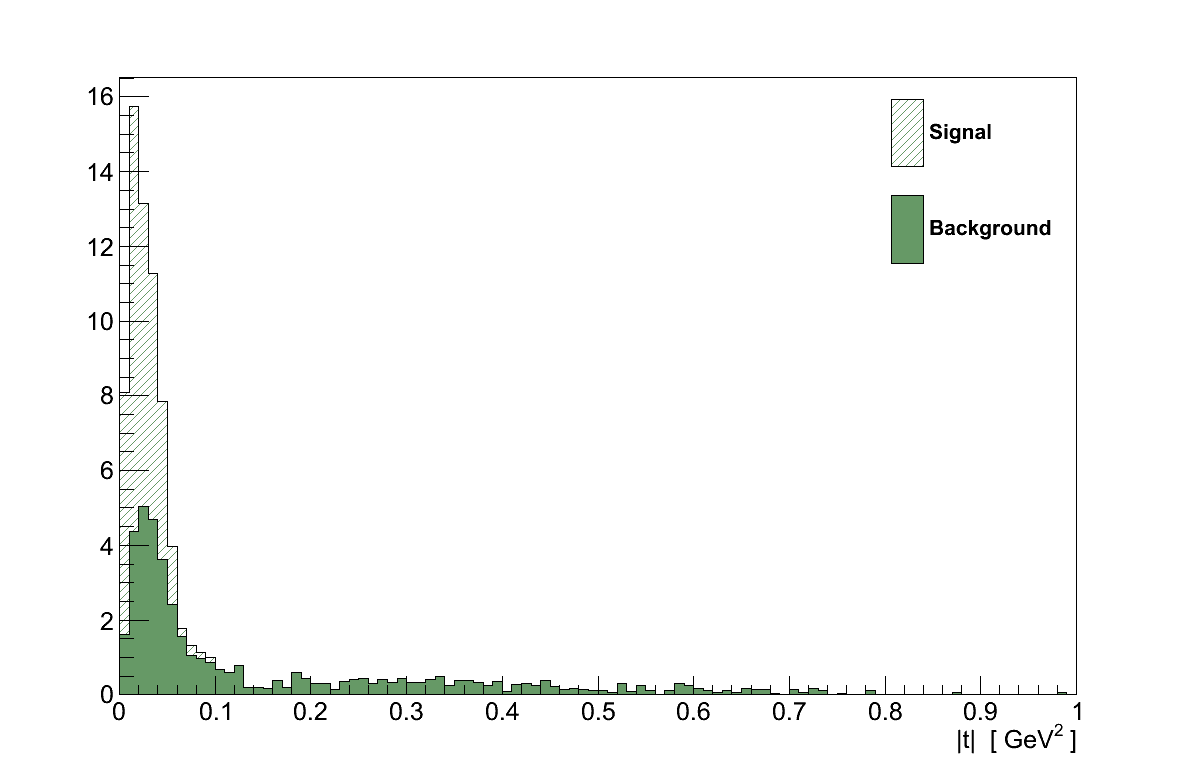
The position of the split between the signal and control regions was set as 0.09 GeV2 by finding the largest possible control region which remains ≥ 99 % background-pure.
The result calculation, which follows a prescription by Glen Cowan et al. [5], begins by taking the counts in each of the two regions measured in data:
- nD - total number of events in signal region
- mD - total number of events in control region
A model of the underlying physics is then constructed using four parameters:
- s - number of signal events in the signal region
- b - number of background events in the signal region
- τ - ratio of background events in signal and control regions
- μ - signal strength, a multiplicative factor which scales s
This model then returns the expected counts in the signal and control region as:
- nE = μs + b
- mE = τb
The likelihood of the measured data being produced by a given choice of model is then the product of Poisson probabilities for the counts, and a Gaussian probability for τ compared with its nominal value and uncertainty:
This is more convenient to calculate by taking the natural logarithm which, up to a constant which is irrelevant for maximisation and will cancel in a forthcoming ratio, is approximately:
Using this definition, the model can be fit to the data by finding the values of the parameters which maximise the likelihood.
In this analysis the signal count in the signal region, s, is taken directly from that predicted in simulation and kept constant throughout (i.e. it was not allowed to vary during fitting). It is the signal strength, μ, which allows its contribution to vary. The simulation also provides the value of τnominal. The uncertainty on τnominal, στ, will be determined in Section 6.10, and represents the sole source of systematic uncertainty.
In general, when maximising the likelihood the values of b, τ and μ are allowed to vary. The first term in Equation 6.9 measures the degree of agreement in the signal region - the principle measure of how well the model describes the data. Meanwhile, the second and third terms in Equation 6.9 control the expected background in the signal region. Though b is allowed to vary, the data count in the control region, mD, constrains it in the second term, since b = mE/τ. While some freedom is allowed for the value of τ to vary from the nominal value predicted in simulation, the third term penalises large excursions relative to the uncertainty on it.
This is an important feature of the calculation that's worth emphasising. The result is independent of the absolute normalisation of the background in simulation. Only the shape of the background, between the signal and control regions, is taken from simulation. It is the data in the control region, mD, which provides the background normalisation.
With the likelihood defined, and the procedure for maximising it determined, there are three statistical tests which could be made for this analysis:
-
Search for an excess. This is the primary output of the analysis, measuring the significance of any excess found above the background prediction.
Using Equation 6.8 the likelihood of a given set of model values producing the observed data can be calculated. Fixing the signal strength according to a hypothesis, and allowing the remaining parameters to vary until they maximise the likelihood gives the maximum likelihood of that hypothesis producing the data. But this does not reveal how good a match that hypothesis is relative to others.
To do this a measure of how well a hypothesis fits the data relative to the best possible fit, the maximised likelihood-ratio, is calculated:
(6.10)Here, the presence of a prime on μ, τ or b indicates that the value of those parameters are those which maximise the likelihood. So L(μ′,τ′,b′) takes the values of μ, τ and b which best-fit the data, while L(μ,τ′,b′) is calculated at the value of τ and b which best describes the data for a given value of μ.
When testing the background-only hypothesis, it must be determined how significant any deviation of μ′ from 0 is. To do this the value of ln λ(0) from data can be compared with the distribution of values that would be expected. So called “pseudo-experiments” are generated by drawing randomised values for mD, nD (from Poisson distributions with means mE and nE respectively) and τ (from a Gaussian distribution centred at τnominal with width στ). For each pseudo-experiment the value of ln λ(0) is then calculated. The resulting distribution is that to be expected if the background-only hypothesis were true. Taking the fraction of pseudo-experiments with ln λ(0) greater than that measured in data is a P-value for the data, which indicates the compatibility of the data with μ = 0 (a smaller P-value indicating a more significant excess).
This P-value can be converted to a more intuitive statistical significance by finding the number of standard deviations at which a normal distribution gives that same P-value. The larger the value of this significance the stronger the indications that there is an excess of data in the signal region.
-
Set an upper-limit. In the case that no significant excess is observed, it would be interesting to calculate the largest possible signal strength which could still produce a result that is compatible with the background.
By generating the ln λ(μ) distribution with pseudo-experiments, the P-value for the distribution below the value from data indicates how compatible such a signal strength would be with the background. A 90 % upper-limit, for example, can then be set by finding the largest value of μ for which this lower P-value is 0.9.
-
Measure the signal strength. In the case that a significant excess is found, the signal strength which best matches the data can be found trivially. It is the value of μ′ from the denominator in Equation 6.10, where all the free parameters were allowed to vary to find the maximum likelihood.
Using this procedure it is possible to assess the significance of any excess of events found in the coherent selection, and to provide some interpretation of that significance whether it is large or small. It is important to note however, that any interpretation made of the significance, is done in the context of the coherent model which provided the value of s.
Before proceeding with the result calculations, there is one remaining undetermined input: the uncertainty on the background ratio, στ, through which systematic uncertainties enter into the analysis.
6.10. Systematic Uncertainties
Systematic uncertainties deal with uncertainty in the accuracy of the simulation at describing the data, and therefore reflect variation that can result from differences between the two. For this analysis they can be classified under three categories:
- The flux systematic is a result of uncertainties in the predicted neutrino flux at ND280.
- Interaction systematics deal with uncertainties in the models contained within GENIE, including the nuclear model, neutrino interaction cross-section models and final-state interaction models.
- Detector systematics deal with uncertainties stemming from the simulation of the experiment, including the description of the detector and magnetic fields, the passage of particles through the detector and the response of the detector's electronics to the energy deposited.
In some cases these systematics can be studied by the variation of underlying parameters in the models used, in others they come from studying the possible variations on the resulting properties which are measured. Regardless, systematic uncertainties only affect the analysis when they cause changes in the value of τ, the nominal value of which is τnominal = 1.43. For the systematics studied below, only background events are used, and only changes in the shape of the backgrounds need be considered.
6.10.1. Flux Systematic
The systematic uncertainty in the predicted neutrino flux is assessed by the T2K Beam group, predominantly using NA61/SHINE data, and provided to analysers in the form of a covariance matrix binned by neutrino flavour and energy [6].
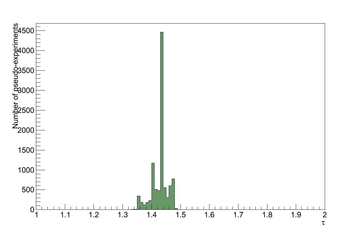
In order to assess this effect, the analysis was re-run 10000 times. Each time the analysis was re-run, weights for each neutrino flavour-energy bin were generated according to the size and correlations of the uncertainty in each bin described by the covariance matrix. Every event was given a weight based on the flavour and energy bin to which the initial neutrino belonged, effectively simulating the effect of a variation in the flux. In each re-run the value of τ was calculated and recorded.
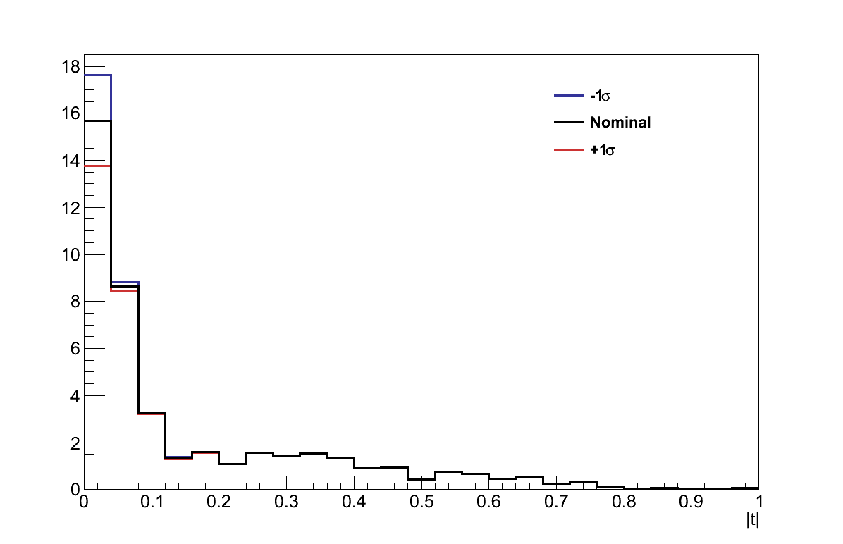
A Gaussian fit was made to the resulting distribution of τ values (Figure 6.18), and the systematic uncertainty from the flux taken to be the standard deviation, στFLUX = 0.042.
6.10.2. Interaction Systematics
As discussed in Chapter 3, there is a great deal of uncertainty in our knowledge of neutrino interaction physics. As a consequence the models used in interaction simulations, such as the GENIE simulation [7] used in this analysis, also carry a great deal of uncertainty with them.
The GENIE simulation provides re-weighting tools which, for a given neutrino interaction, calculate weights corresponding to the effect of varying the values of underlying parameters used in GENIE's models. The GENIE collaboration have also determined estimates of the uncertainties on these model parameters, by comparing the outputs from GENIE under variations of those parameters with a large body of experimental data. The GENIE models and their parameters are described in detail in its user manual [8] and the value of the uncertainties placed on each parameter are discussed along with the procedure by which they are treated in a T2K technical note [9].
Most of the parameters can be classified as belonging to the models for the basic cross-sections (GXSec), the creation of hadrons from fragmented nucleons (GHadr), the interactions of final-state particles as they travel through the nucleus (GINuke), or the decay of particles within the nucleus (GRDcy).
For some parameters GENIE provides two alternatives for the study of their effects. For example the axial mass (MA) in the CC QE model can either be studied directly as a single parameter, or by decomposing its effects to two separate parameters - one for the effect on normalisation of the CC QE cross-section, and one for the effect on its Q2-shape. In such instances, only the combined single parameters were used in this study.
Software developed within the T2K collaboration, “T2KReWeight” [10], provides an interface to the GENIE re-weighting functionality, allowing the re-weighting of simulated neutrino interactions selected in ND280 analyses.
The procedure adopted for assessing the effect of the uncertainty on these parameters was to run the analysis twice for each parameter, once varying that parameter by +1σ, and once varying it by -1σ. In each case, T2KReWeight was used to retrieve weights for the true interaction selected in the analysis, and that weight was applied to the event. Figure 6.19 shows the effect on the |t| distribution of re-weighting in this way, for examples of four of the more significant parameters.
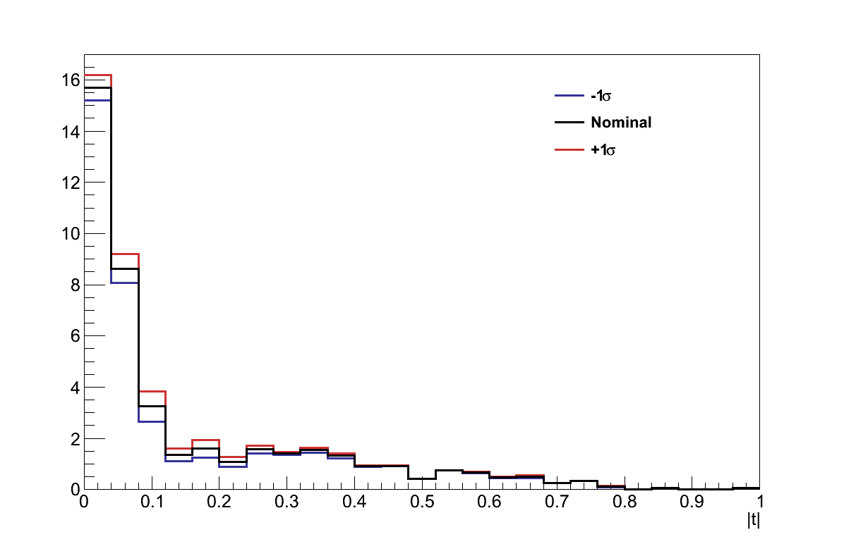
The values of τ resulting from this re-weighting were then calculated for the two shifts of each parameter, and are shown in Figure 6.20 for the parameters which affected the analysis. For each parameter, the largest shift in the value of τ was taken to be the uncertainty from that parameter. The total uncertainty resulting from the interaction modelling was then taken from the sum-in-quadrature of all the parameters: στINTERACTIONS = 0.398.
| Parameter Name | Parameter Description | σ [%] |
|---|---|---|
| GXSec_MaCCQE | Parameter in CC QE axial form-factor | 25 |
| GXSec_VecFFCCQEshape | Choice of CC QE vector form-factors (BBA05 / dipole) | - |
| GXSec_MvCCRES | Parameter in CC resonance vector form-factor | 10 |
| GXSec_MaCCRES | Parameter in CC resonance axial form-factor | 20 |
| GXSec_MvNCRES | Parameter in NC resonance vector form-factor | 10 |
| GXSec_MaNCRES | Parameter in NC resonance axial form-factor | 20 |
| GXSec_RvpCC1pi | Non-resonance ν CC 1π | 50 |
| GXSec_RvpCC2pi | Non-resonance ν CC 2π | 50 |
| GXSec_RvnCC1pi | Non-resonance ν CC 1π | 50 |
| GXSec_RvnCC2pi | Non-resonance ν CC 2π | 50 |
| GXSec_RvnNC1pi | Non-resonance ν NC 1π | 50 |
| GXSec_RvnNC2pi | Non-resonance ν NC 2π | 50 |
| GXSec_RvbarpCC1pi | Non-resonance ν CC 1π | 50 |
| GXSec_RvbarpCC2pi | Non-resonance ν CC 2π | 50 |
| GXSec_RvbarnCC1pi | Non-resonance ν NC 1π | 50 |
| GXSec_AhBY | AHT parameter in Bodek-Yang (DIS) model scaling variable ξW | 25 |
| GXSec_BhBY | BHT parameter in Bodek-Yang (DIS) model scaling variable ξW | 25 |
| GXSec_CV1uBY | CV1u u-quark valence GRV98 PDF correction parameter in Bodek-Yang (DIS) model | 30 |
| GXSec_CV2uBY | CV2u u-quark valence GRV98 PDF correction parameter in Bodek-Yang (DIS) model | 40 |
| GHadrAGKY_xF1pi | Pion Feynman-x PDF for Nπ states in AGKY (hadronisation model) | - |
| GHadrAGKY_pT1pi | Pion transverse momentum PDF for Nπ states in AGKY (hadronisation model) | - |
| GHadrNucl_FormZone | Hadron formation zone length | 50 |
| GINuke_MFP_pi | π mean free path (total rescattering probability) | 20 |
| GINuke_MFP_N | Nucleon mean free path (total rescattering probability) | 20 |
| GINuke_FrCEx_pi | π charge exchange probability | 50 |
| GINuke_FrElas_pi | π elastic reaction probability | 10 |
| GINuke_FrInel_pi | π inelastic reaction probability | 40 |
| GINuke_FrAvs_pi | π absorption probability | 20 |
| GINuke_FrPiProd_pi | π probability | 20 |
| GINuke_FrCEx_N | Nucleon charge exchange probability | 50 |
| GINuke_FrElas_N | Nucleon elastic reaction probability | 30 |
| GINuke_FrInel_N | Nucleon inelastic reaction probability | 40 |
| GINuke_FrAvs_N | Nucleon absorption probability | 20 |
| GINuke_FrPiProd_N | Nucleon probability | 20 |
| GSystNucl _CCQEPauliSupViaKF |
CC QE Pauli suppression (via kF) | 35 |
| GRDcy_BR1gamma | Branching ratio for radiative resonance decays | 50 |
| GRDcy_BR1eta | Branching ratio for single-η resonance decays | 50 |
| GRDcy_Theta_Delta2Npi | Choice of pion angular distribution in Δ → πN (isotropic / Rein-Sehgal) | - |
As mentioned, the GENIE manual [8] provides a thorough description of the various models, their parameters and parameter uncertainties. For information, the list of parameters which affect the analysis and their uncertainties are shown in Table 6.9. For the more significant parameters in this analysis the descriptions in the GENIE manual are summarised:
-
Cross-Section Form-Factors
Variations in the form-factors for CC QE and resonance production are simply treated by calculating the differential cross-section for the given interaction with the nominal and alternative values of the parameters. The interaction then simply receives a weight corresponding to the change of the differential cross-section.It is clear that the CC QE axial-mass form-factor parameter (GXSec_MaCCQE) dominates the interaction uncertainty. As can be seen in the bottom-right of Figure 6.19 this is a result of almost all the CC QE background lying within the control region, and hence any changes of their normalisation have a direct effect on τ. This is further exaggerated by the high 25 % uncertainty currently assigned to this parameter, predominantly motivated by the fitting of larger values of MA in MiniBooNE.
-
Inelastic Cross-Sections
As was discussed in Chapter 3, inbetween the regions dominated by resonance and DIS interactions is a “transition region”, where the target nucleon can produce off-shell resonances or is partly fragmented but does not clearly fall into either category.This can be modelled as some combination of resonance and DIS models, but simply summing them would result in double-counting. In GENIE this is treated by combining the resonance model with a scaled and modified version of the DIS model below a threshold in invariant hadronic mass (W < 1.7 GeV). In this region the DIS contribution is:
(6.11)Where m refers to the initial state and the multiplicity of the hadronic system (m = νpCC1π, νpCC2π, νnNC1π…), and Pm is the default probability of that final hadronic system from the hadronisation model. The Rm are then tunable parameters which scale each of the different components. The values of the Rm, and uncertainties on them, are set by the GENIE collaboration by fitting data on inclusive, 1π and 2π final-states from multiple experiments.
The uncertainty in these Rm parameters are controlled in the re-weighting by the parameters beginning “GXSec_R”. As is to be expected, the uncertainty on those parameters which relate to final states containing pions are those which affect this analysis the most, in particular GXSec_RvnCC1pi which for νμ corresponds to the production of μ- + π+ topologies.
-
INTRANUKE
The INTRANUKE/hA model is the intra-nuclear rescattering model implemented in GENIE, which determines the effect on hadronic particles of propagating out through the nuclear environment. During this propagation particles may undergo elastic scattering, inelastic scattering, charge exchange or absorption. The model has been extensively tuned on scattering data from other fields, particularly hadron-nucleus scattering and photon-nucleus scattering.Essentially the INTRANUKE/hA model selects either survival or rescattering as the fate of a hadron (h = π,N) at δr = 0.05 nm steps acording to the probabilities calculated:
(6.12)Where r is the position of the hadron within the nucleus, and λh is the mean free path of that hadron, which is a function of its position and energy, E:
(6.13)With ρ the nuclear density, and σhN the total interaction cross-section for that hadron with a nucleon.
If the hadron is determined to rescatter at any point an interaction mode is chosen according to the relative sizes of their respecitve cross-sections (see Figure 6.21). The fate of hadrons simulated to result from that interaction must also then be calculated.
Figure 6.21: For hadrons determined to undergo rescattering in INTRANUKE/hA, the fractions of each scattering mode available to them as a function of their kinetic energy, for pions (left) and nucleons (right) [9]. The re-weighting paramaters beginning “GINuke_MFP” modify the mean free paths, λh acording to the uncertainty assigned to them from the data tuning mentioned earlier. An event then receives a weight which is the product of weights assigned to each of the primary hadrons generated at the neutrino interaction vertex. The weight given to each primary hadron is calculated from the change in its survival probability. If Psurvive increases for a hadron which did survive it is weighted up. If Psurvive decreases for a hadron which did survive it is weighted down. The inverse is applied to primary hadrons which did not survive.
The re-weighting parameters beginning “GINuke_Fr” alter the fraction of hadron rescatters assigned to each of the possible interaction modes. Again, events are given a weight which is the product of weights assigned to each of its primary hadrons. The primary hadrons receive a weight if their fate was to undergo the interaction, proporitonal to the change in that interaction's fraction.
The intra-nuclear interactions of pions directly affect their number which escape the nulceus, and the intra-nuclear interactions of nucleons can often result in additional pions being created. The fact that many of the INTRANUKE/hA re-weighting parameters strongly affects the background events in this analysis is consistent with expectations.
-
Δ Decay Kinematics
The parameter GRDcy_Theta_Delta2Npi has a significant effect on the analysis. This is unsurprising since it controls the angular distribution of π+ resulting from the decay of Δ resonances, and it is clear that a more forward-peaked distribution would result in lower reconstructed values of |t|.A general expression of the angular distribution, Wπ, of pions from Δ → N π+ [8]:
(6.14)Where p(3/2) and p(1/2) are coefficients, and P2 is the 2nd order Legendre polnomial. The Rein-Sehgal resonance model [11] predicts p(3/2) = 0.75, p(1/2) = 0.25. However, for simplicity, GENIE decays Δs isotropically (effectively p(3/2) = p(1/2) = 0.5).
The effect of re-weighting GRDcy_Theta_Delta2Npi, which corresponds to varying this distribution from isotropy (0σ) to Rein-Sehgal (+1σ) or any step inbetween, is shown in Figure 6.22.
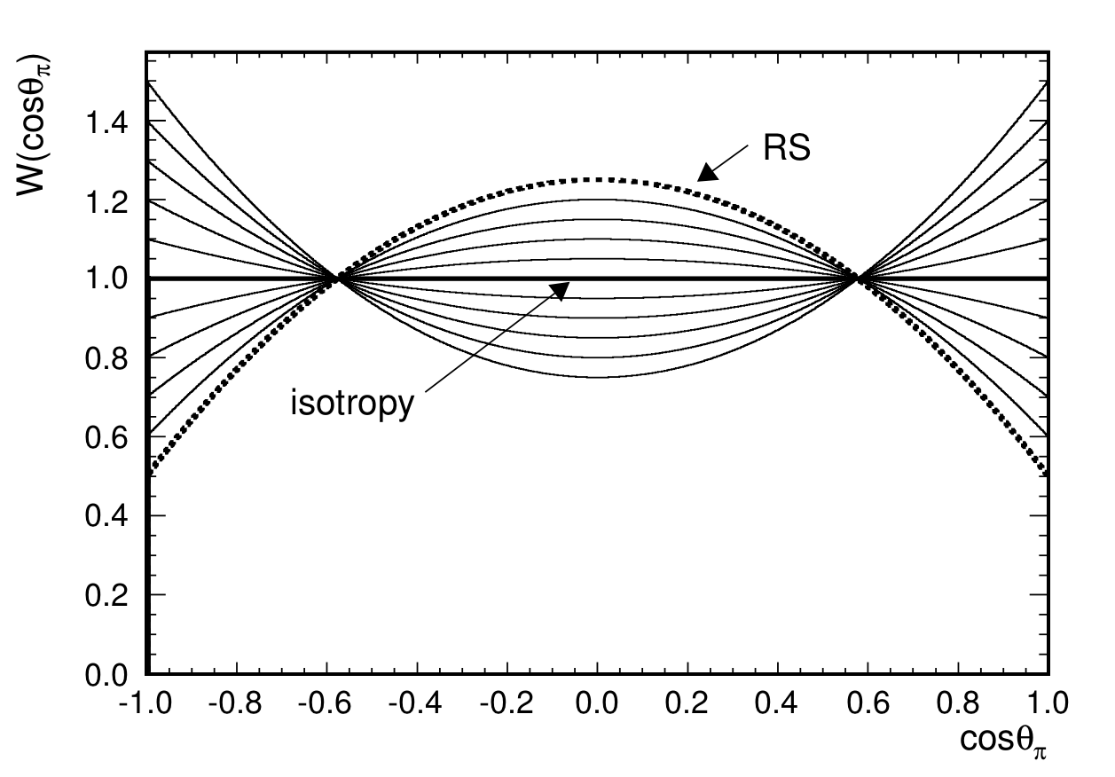
Figure 6.22: The angular distribution of pions resulting from Δ decays for values of GRDcy_Theta_Delta2Npi ranging from -1σ, through 0σ (isotropy), to +1σ (Rein-Sehgal) [8].
6.10.3. Detector Systematics
There are numerous systematic differences in the simulation of the detector that could affect this analysis:
- differences in the reconstruction efficiency, particularly those which are a function of a track's angle or momentum
- differences which affect the measurement of a track's properties, particularly its direction or momentum
- differences in the passage of particles through the detector, particularly when it affects their ability to make reconstructible tracks
- differences in the measurement of energy deposited at the vertex
The categorisation, treatment and quantification of the detector systematics here broadly follows that which was done for the ND280 νμ Inclusive analysis [1] [2] and its supporting studies.
6.10.3.1. Momentum Resolution
There are two potential sources of systematic difference in the reconstructed momentum of a track: the absolute value of the measurement, and the resolution of the measurement.
The reconstruction measures a track's momentum from the component of the momentum transverse to the magnetic field, pB. The resolution on 1/pB is approximately Gaussian and, as mentioned in Section 6.2, it is found that this is 32 ± 10 % worse in data than in simulation. A correction was applied to account for the 32 % difference, so the remaining uncertainty on the momentum resolution is σ(1/pB) = 10 % [4].
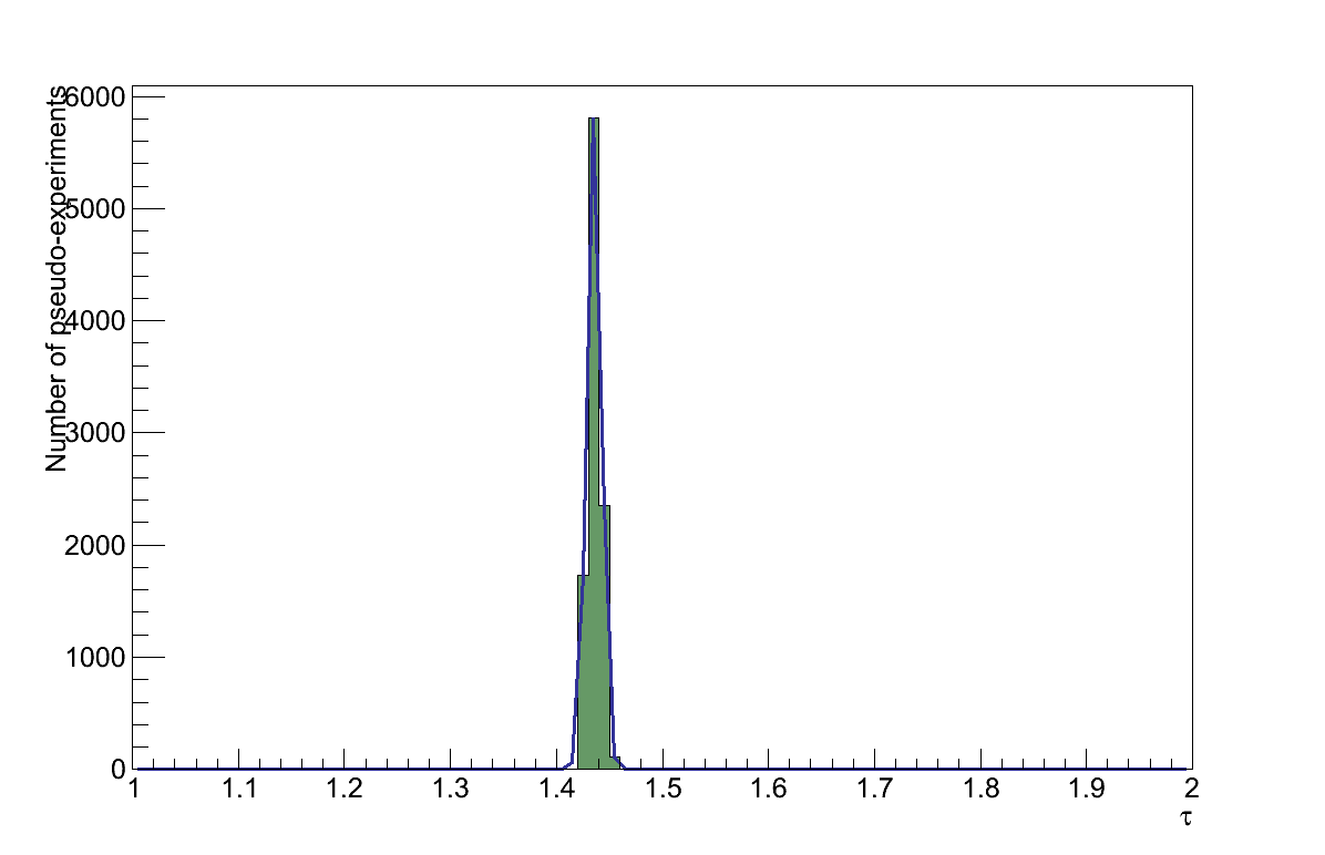
To assess the effect of this uncertainty, the analysis was re-run 10000 times, each time selecting a new resolution, δσ, from a Gaussian centred at 1.0 with width 0.1. The muon and pion tracks' 1/pB were then adjusted based on this change of resolution in the same way as the initial correction (Equation 6.1):
The tracks' reconstructed momentum was then updated based on the new value of 1/pB, and the resulting value of τ recorded. The resulting distribution was non-Gaussian with quantised spikes as a result of events migrating across the pT cut (Figure 6.23). Since a Gaussian fit cannot be made to this distribution, the largest deviation in the value of τ was taken to be the uncertainty from the momentum resolution: στP-RESOLUTION = 0.084.
6.10.3.2. Momentum Scale
The second possible systematic difference in the momentum can come from the absolute scale of the measurement, which is dominated by uncertainty in the strength of the magnetic field. Using measurements of the magnetic field taken with Hall probes inside ND280, the uncertainty on the magnetic field strength is found to be 0.5 %[12].
To assess the effect of this uncertainty, the analysis was re-run 10000 times, each time selecting a new scale factor from a Gaussian centred at 1.0 with width 0.005. The muon and pion tracks' momentum were then scaled according to this factor, and the resulting value of τ recorded. A Gaussian fit was made to the resulting distribution of τ values (Figure 6.23) and the uncertainty from the momentum scale taken from its width: στP-SCALE = 0.0069.
6.10.3.3. FGD-TPC Matching
In order to enter this analysis, the ND280 reconstruction must successfully match the reconstructed tracks left by the muon in FGD 1 and TPC 2. If the efficiency, ε, of this matching differs between data and simulation as a function of momentum or angle, the resulting value of τ could also differ.
Using high statistics samples of cosmic-ray and T2K beam muons, a study of this matching efficiency concluded that the uncertainty on data-simulation agreement for ε did vary as a function of momentum and angle [13]. The study reported matching efficiency uncertainties, σεij, for sixteen bins in muon momentum and angle (four of each, indexed by i and j) with values ranging in magnitude: 0.21 % ≤ σεij ≤ 1.25 %. These uncertainties were stated to be uncorrelated.
To assess the effect of a systematic difference in the matching efficiency between data and simulation, two weights were calculated for each muon momentum-angle bin, corresponding to an increase or decrease in efficiency:
Each momentum-angle bin was then considered independently, twice: once calculating the effect on τ of an increase in efficiency, and once for a decrease. This was done by weighting those events whose muon fell in that momentum-angle bin by the value calculated in Equation 6.16. In each case the shift, δτij(±), in the resulting value of τ was calculated and the magnitude of the largest shift for each bin was taken to be the uncertainty in that bin:
The sum-in-quadrature of all στij was then taken to give the total uncertainty resulting from the FGD 1-TPC 2 efficiency matching as: στMATCHING = 0.0025.
6.10.3.4. TPC Track Quality Cut
Both the selection of the muon and pion candidate tracks include the requirement that they have a “good” component in TPC 2, defined as a TPC 2 track with hits on ≥ 18 of the micromegas' readout columns (the TPC reconstruction is based on initially clustering of hits vertically). A difference in the efficiency of detecting those hits, ε, between data and simulation could result in tracks migrating across this 18 hit cut. If the susceptibility of a track to crossing that cut has a momentum or angle dependence, such a difference could also result in a change in τ.
A comparison of the number of vertical clusters between data and simulation was made for muon candidate tracks from the νμ Inclusive selection, where the track crossed two micromegas in TPC 2 (≥ 62 vertical clusters). The difference in hit efficiency between data and simulation was then found by modelling the effect of such a difference on the distribution from simulation, and fitting the data distribution. A variety of studies as a function of location, momentum, angle etc. concluded that in all cases the difference in hit efficiency [13]:
Since this difference is small only the loss of a single hit is sufficiently likely to change the event selection. The effect of a lower efficiency in data is assessed by giving each track with exactly 18 vertical clusters in TPC 2 a weight of 1 - Δε = 0.999, and every other track a weight of 1.0. Each event is then given a weight from the product of its two tracks' weights, and the resulting shift in the value of τ calculated. The effect on τ of an increase in efficiency is assumed to be symmetric to that from a decrease, allowing the calculated shift to be taken as the systematic uncertainty resulting from the TPC track quality cut: στQUALITY = 0.00004.
6.10.3.5. Out of Fiducial Volume Backgrounds
There are broadly three sources of backgrounds originating outside of the fiducial volume (OOFV): cosmic ray muons, “sand muons” from interactions upstream of ND280, and interactions within ND280 but outside the fiducial volume.
The νμ Inclusive analysis estimated that they would select 3 events from cosmic rays over T2K Runs 1-3 (0.02 % of their events). Since it is highly unlikely that these events could also produce a track meeting the requirements of the pion candidate, and pass the subsequent analysis cuts, no systematic was assigned due to cosmic ray backgrounds.
Interactions of beam neutrinos upstream in the sand surrounding the ND280 facility are not included in the standard ND280 beam simulation but are simulated in a standalone production. Applying the coherent pion selection to this sample, equivalent to 12×1020 POT, resulted in zero events being selected, so no systematic uncertainty was applied due to sand muon backgrounds.
The only remaining source of OOFV backgrounds are those from interactions elsewhere in ND280, which make up just 2 % of the simulated events selected. These events fall into three categories: interactions in the FGD 1 scintillator bounding the fiducial volume (32 %), interactions in the Tracker dead-material (26 %) and interactions outside the tracker (42 %).
The uncertainty in the rate of these backgrounds coming from interaction and flux simulations has already been taken into account. This leaves two possible sources of systematic differences: differences in the mass of the regions in which the interactions take place, and differences in the reconstruction effects which allowed them into the selection.
A study conducted for the νμ Inclusive analysis concluded that no additional reconstruction uncertainty for OOFV backgrounds in the FGD 1 scintillator or Tracker dead-material need be considered beyond those already dealt with. Interactions from outside the Tracker however, which likely entered FGD 1 at high-angle, were assigned a 45 % reconstruction uncertainty [14].
The difference in mass between the real and simulated FGD 1 scintillator is 0.009 %, while the difference in mass of the entire detector is 0.67 % [15]. The former is therefore taken as the uncertainty on FGD 1 scintillator OOFV background, and the latter is taken as the uncertainty on interactions in the Tracker dead-material.
For the mass uncertainty for interactions outside the Tracker, a value of 10 % is estimated based on the uncertainty in the mass of the ECal detectors. This value originates primarily from the 10 % tolerance on the thickness specified by the supplier of the lead sheets which dominate the total mass of the ECals. From my work writing the simulation of the ECal detectors, I believe this uncertainty also covers the differences in the ECal's surrounding dead material.
The total uncertainties for the OOFV interactions are then: 0.009 % for interactions in FGD 1 scintillator, 0.67 % for interactions in Tracker dead-material, and 46 % for interactions outside the Tracker (from the sum-in-quadrature of the mass and reconstruction uncertainties).
To assess the effect of OOFV interactions on the value of τ, the analysis was re-run twice for each of the three categories described above, weighting the corresponding interactions up and down according to the uncertainty assigned to them. For each category, the largest of the two resulting shifts in the value of τ is taken to be the uncertainty resulting from that category. Finally, the total OOFV uncertainty is taken from the sum-in-quadrature of the three categories' uncertainties, giving a value of: στOOFV = 0.0079.
It should be noted that the OOFV fraction in the selection is very small - totalling only 31 raw interactions in simulation. As a result the size of the statistical uncertainty in this sample is significant relative to the systematic uncertainty. Any future analysis which had access to greater simulation statistics would therefore want to re-evaluate this systematic. As will be seen in Section 6.10.4 however, such uncertainty is of little consequence for this analysis.
6.10.3.6. Pion Interactions
Another potential systematic difference between data and simulation is in the passage of charged pions through dense matter, such as the scintillator of FGD 1. There is evidence to suggest that the cross-sections for interactions which would prevent a π+ from leaving FGD 1 are not well simulated by GEANT4, which is used in the ND280 simulation. The interactions which could most directly prevent a π+ from leaving FGD 1 are absorption (where the pion is captured by a nucleus) and charge exchange (where a nuclear interaction results in the π+ being replaced by a π0).
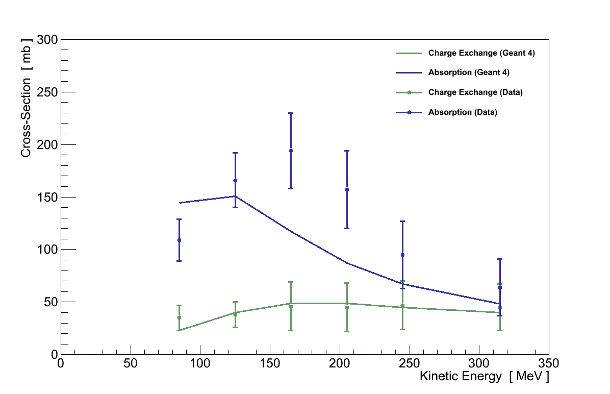
The effect of such a difference on this analysis was determined by adapting a similar study conducted for the νμ Inclusive selection [16], which compared the π+ interaction cross-sections in carbon from GEANT4 with published experimental values (Figure 6.24). The goal is to consider the effect that higher or lower cross-sections would have on π+ which made it into TPC 2 and were selected by this analysis.
First, a sample of π+ which had the potential to enter TPC 2 and contribute to the analysis was selected by searching events in the νμ Inclusive selection for those which meet the following requirements:
- The number of π+ made in the simulated interaction was exactly 1
- A linear extrapolation of the initial direction of the π+ to the back of FGD 1 indicates it would enter TPC 2.
(At z = 446.955 mm: |x| ≤ 874.51 mm, |y - 55.0 mm| ≤ 874.51 mm)
Each of these interactions was then classified according to the fate of the π+:
- Underwent charge-exchange (CE)
- Underwent absorption (ABS)
- Entered TPC 2 (TPC2)
- Other
The method for classifying a pion as undergoing charge exchange or absorption followed that defined in the original pion interactions study [16]. Pions were determined to have entered TPC 2 if they were labelled as having done so by the simulation, and all remaining events were classified as other. This final category contains pions which underwent interactions other than charge exchange or absorption which resulted in them not entering TPC 2, or where the simple linear extrapolation was misleading. All of the selected interactions were then binned in 2D histograms, one for each category, according to the initial kinetic energy of the pion, Tinit, and its extrapolated distance from TPC 2.
For those events in the charge exchange or absorption categories, the final kinetic energy of the pion, Tfinal, at the point it interacted was also estimated, again following a procedure defined in the original study2Essentially, the Bethe-Bloch formula was used to calculate the energy lost over the distance from creation to absorption/charge exchange.. Using Tfinal the cross-sections for data and simulation were found by linearly-interpolating the information shown in Figure 6.24. Weights corresponding to taking the simulated cross-section to the top, w+, and bottom, w- of the data's uncertainty band were then calculated for these events, and used to fill two additional weighted histograms for each category.
The total number of pions in each Tinit-distance bin (ij) can be calculated from the un-weighted histograms:
The total number of pions is constant, and it is assumed that the “other” category is unaffected by changes in the pion cross-sections. Then the re-weighted number of pions in the TPC 2 category can be calculated corresponding to the top, NTPC2,+, and bottom, NTPC2,-, of the data uncertainty bands using the contents of the weighted charge exchange and absorption histograms, in every bin:
Finally, weights equivalent to such changes in the pion interaction cross-sections can also be calculated for each bin:
An example of the resulting weights, calculated for the top of the data uncertainty band, is shown in Figure 6.25.
Now, the effect on the value of τ can be determined by re-running the analysis twice, once for each of the top/bottom data uncertainty band weights. For every event where the pion candidate track corresponded to a true pion, the event was given the weight calculated in Equation 6.21 for a pion with that Tinit-distance. Taking the largest of the two resulting shifts in the value of τ, the uncertainty due to pion interactions was calculated as: στPION = 0.039.
6.10.3.7. Vertex Activity
The final systematic to be considered is that for the vertex activity (VA), which is directly cut on in the analysis (Section 6.7). Differences in the amount of energy deposited by particles, or in the response of the detector to a given energy deposition could result in differences in the VA measured.
The FGD group assessed the level of agreement in the energy recorded by FGD 1 for two samples of particles from data and simulation. For muons, which generate relatively low energy hits, the distribution of energies deposited in hits was found to agree within 3 %. For stopping protons, which generate very high energy hits, there was found to be an approximately 10 % shift in the 3×3 vertex activity3Unlike this analysis, which uses a 5×5 region of bars, the stopping protons study used a 3×3 region of bars as the vertex activity. measured at the end of the track (Figure 6.26) [17].
The 5×5 VA cut of 290 PEU corresponds to an average hit energy between these two extremes. However, since the VA is cut on directly, and the distribution of hit energies could include high fluctuations, the uncertainty assigned to the VA was set to 10 %.
To assess the effect of the VA uncertainty on the value of τ the analysis was re-run twice, once scaling the VA for each event up by 10 %, once scaling it down by 10 %. Each time the value of τ was recalculated, and the largest of the two resulting shifts was taken as the uncertainty due to the VA: στVA = 0.073.
6.10.4. Summary
Table 6.10 shows a summary of all the systematic uncertainties considered. The individual absolute uncertainties were combined via a sum in quadrature to conclude that there is a total 29 % systematic uncertainty: τ = 1.43 ± 0.42.
| Source | Uncertainty | ||
|---|---|---|---|
| Absolute | Fractional | ||
| Flux | 0.042 | 2.9 % | |
| Interactions | 0.398 | 27.8 % | |
| Detector | Momentum resolution | 0.084 | 5.8 % |
| Momentum scale | 0.0069 | 0.48 % | |
| FGD-TPC matching | 0.0025 | 0.17 % | |
| TPC track quality cut | 0.00004 | 0.003 % | |
| OOFV | 0.0079 | 0.55 % | |
| Pion interactions | 0.039 | 2.7 % | |
| VA | 0.073 | 5.1 % | |
| Total | 0.42 | 29.1 % | |
6.11. Results
Figure 6.27 shows the |t| distribution for events selected in data and simulation. In the signal region, |t| < 0.09 GeV2, there are 53 events in data, compared with a prediction of only 25.3 background events from simulation. In the control region there are 12 data events, compared with 17.6 in simulation.
The event numbers in the two regions from data and simulation are summarised in Table 6.11. It is these numbers which are input into the result calculations.
| Data | Signal region, nD | 53 |
|---|---|---|
| Control region, mD | 12 | |
| Simulation | Signal region, s | 39.0 |
| Signal region, b | 25.3 | |
| Control region, b / τnominal | 17.6 | |
| τnominal | 1.43 ± 0.42 |
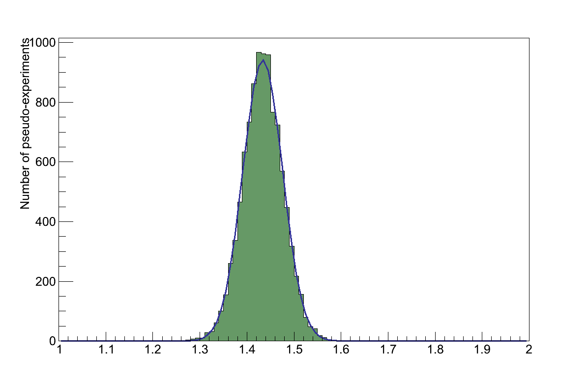
The first calculation is a comparison of the data to the “background-only hypothesis”, the assumption that there is no coherent signal (μ = 0) and only background events. A sample of 10 million pseudo-experiments were generated to find the maximised log-likelihood ratio distribution, which is shown in Figure 6.28 compared with the maximised log-likelihood ratio of the data: ln λ(0) = 5.35.
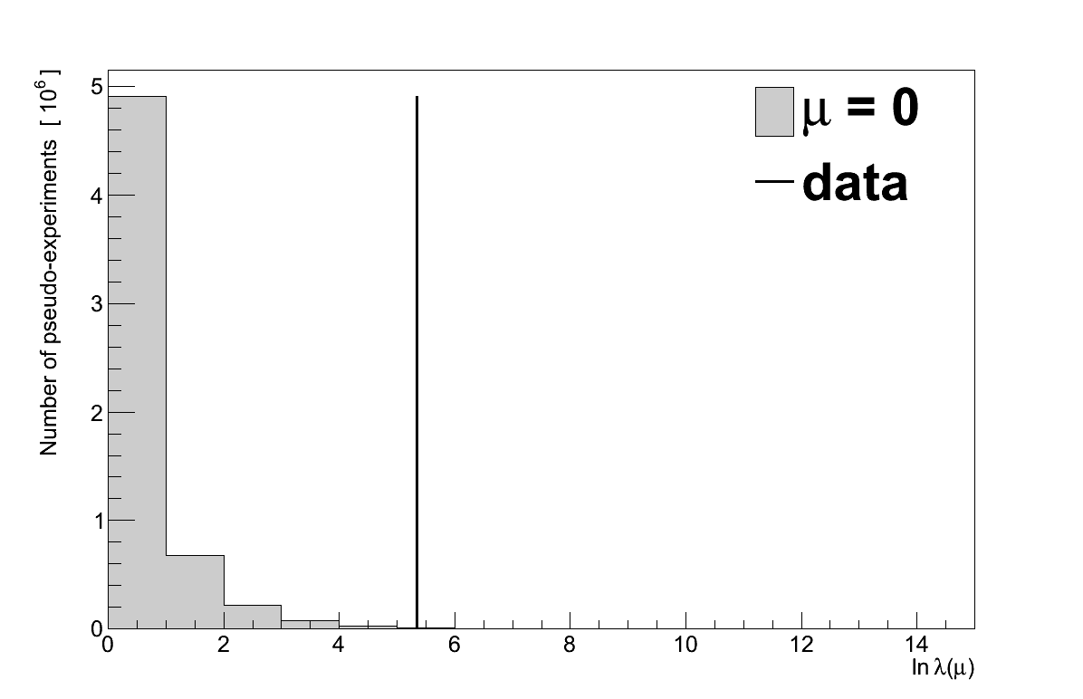
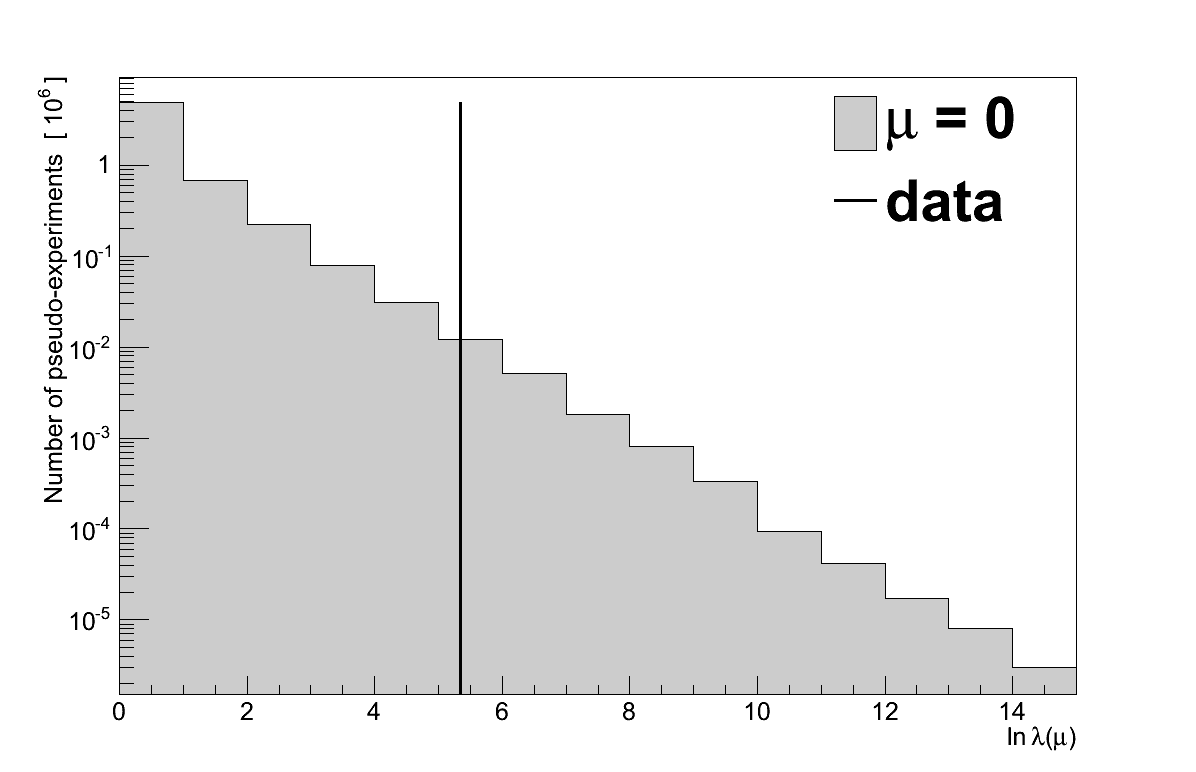
In 13371 pseudo-experiments the value of ln λ(0) was ≥ 5.35, giving the data a P-value of 0.00134. Converted to a significance, that corresponds to a 3.003 σ excess.
The stringent limits set on the existence of νμ CC coherent pion production by SciBooNE motivated this analysis to be conducted as a search rather than a measurement. None the less, faced with such a significant excess it is interesting to explore what this result says if considered as a signal from coherent pion production.
As discussed in Chapter 4, it is widely believed that an alternative to the Rein-Sehgal model will be required to successfully describe coherent pion production at these low neutrino energies. However its implementation in the GENIE simulation used in this analysis, and its wide use in other analyses, provide a good baseline with which to interpret the data.
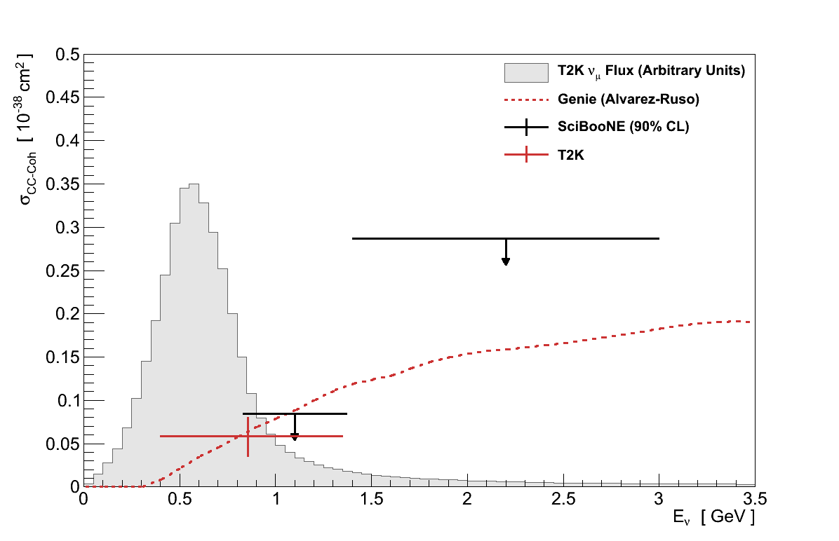
The maximised likelihood, L(μ′,τ′,b′), found in the result calculation gives the values of μ and τ which best describe the data, i.e the best-fit signal-strength4The uncertainties on this value come from statistics and τ. They do not include systematic uncertainties on the signal efficiency.. For the GENIE simulation this is found at μ′ = 0.92 +0.34-0.36. In other words, the Rein-Sehgal model in GENIE would best describe the data if its cross-section were 92 % of the default.
For a cross-section σ(Eν) and flux Φ(Eν), the flux-averaged cross-section is defined:
Applying the best-fit signal-strength to the GENIE Rein-Sehgal model averaged over the νμ flux at ND280 gives a flux-averaged cross-section:
For reference, this measurement was made on a predominantly carbon target with Aeffective = 12.10 (Section 5.4.2), in a νμ beam with mean energy 0.856 GeV, and where 68 % of the total νμ flux is found within 0.475 GeV of that mean.
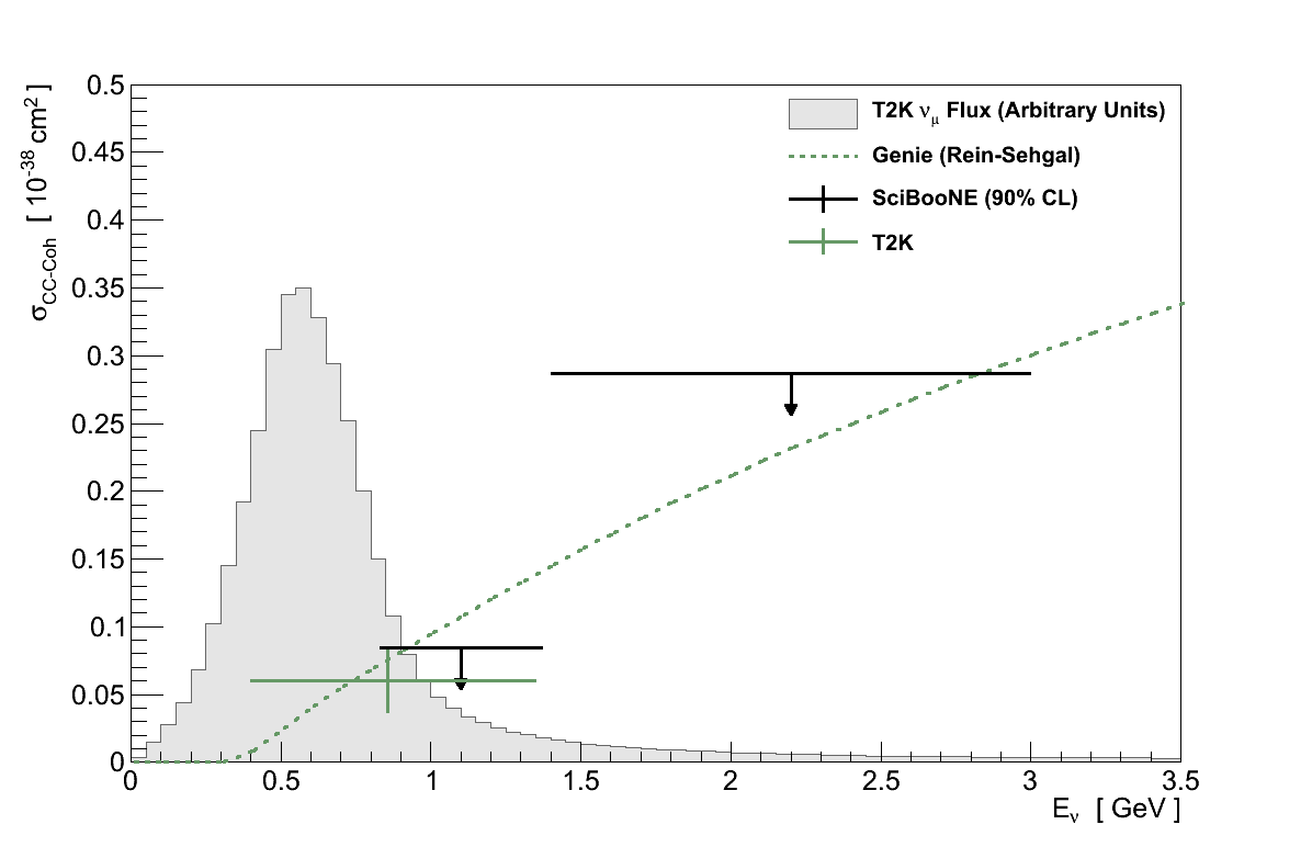
Figure 6.29 shows this result compared with the limits set by SciBooNE, along with the default Rein-Sehgal cross-section in GENIE.
6.11.1. Comparison with the Alvarez-Ruso model
The analysis was re-run using the Alvarez-Ruso model implemented in GENIE. Recalling Section 6.2, this sample used the same background events from the standard GENIE simulation, and all cut values were left the same. Its purpose being to assess how dependent the analysis is on the coherent model used.
Table 6.12 shows the effect on signal events of the various selections and cuts in the analysis, compared between the Rein-Sehgal and Alvarez-Ruso models. The efficiencies from the two models are very similar at every stage of the analysis and, most importantly, differ by just 1 percentage point at the final selection. This is consistent with the analysis goal of being as model independent as possible.
| Step | Data | Rein-Sehgal | Alvarez-Ruso | ||||
|---|---|---|---|---|---|---|---|
| Total | Signal | Efficiency | Total | Signal | Efficiency | ||
| νμ Inclusive selection | 10303 | 10016 | 96 | 78 % | 9983 | 63 | 74 % |
| Coherent Initial selection | 620 | 704 | 52 | 42 % | 689 | 38 | 44 % |
| pT cut | 122 | 169 | 43 | 35 % | 156 | 30 | 35 % |
| VA cut | 65 | 81 | 39 | 32 % | 71 | 28 | 33 % |
Figure 6.30 shows the distributions on which the two cuts are placed. For the transverse momentum distribution (cf. Figure 6.13) the Alvarez-Ruso model predicts a very simlar distribution to Rein-Sehgal model, after accounting for the overall difference in normalisation. The vertex activity distribution (cf. Figure 6.15) is also very similar between the two models. This is to be expected since the VA measured for coherent events is mostly independent on the kinematics of the muon and pion created.
The kinematics of the muon and pion candidates from the final selection are shown in Figure 6.31 (cf. Figure 6.16). The angular plots show the Alvarez-Ruso model's preference for more forward-going topologies, though the difference in this flux-integrated distribution is more slight than the comparison at fixed energy in Section 4.3. The pion momentum spectrum is also noticable softer, with fewer events exceeding 1000 MeV than for Rein-Sehgal. Comparing the four plots in Figure 6.31 and Figure 6.16, neither model is consistently the better at describing the data. Given also the degree of uncertainty on the background events lying underneath, no statement can be made on which model is preferred.
The |t| distribution of the Alvarez-Ruso model shown in Figure 6.32 (cf. Figure 6.27), again shows its slight preference for a more forward-going topology. However, because this difference moves events further from the cut value, it does not adversely affect the analysis.
Since the background events in this simulation are identical to those in the standard GENIE simulation, there is no need to repeat the search for an excess. In fact the only fit parameter that differs from the standard GENIE simulation is the signal prediction, s = 27.8. Calculating the best-fit signal strength, μAR = 1.28+0.48-0.51, which gives a best-fit flux-averaged cross-section of5Please note that the model used here is not identical to the authors' full model (see Section 4.3).:
This best-fit signal strength is in remarkable agreement with the data, though considering the size of the uncertainty on it no strong conclusion can be drawn from it. The best-fit fluz-averaged cross-section is compared with the default Alvarez-Ruso cross-section and SciBooNE limits in Figure 6.33.
6.11.2. Comparison with NEUT
The analysis was also re-run using the NEUT simulation generated as part of the production 5 processing. Since the Rein-Sehgal model in NEUT is quite dated the motivation for reviewing it is its relevance for other ND280 analysers who use NEUT as their primary simulation, and its alternative background model.
Table 6.13 shows the number of total and background events at each stage in the analysis, compared between GENIE and NEUT. It is clear that NEUT predicts quite different background numbers compared to GENIE. Although its total event prediction agrees better with data early on, that trend is gradually reversed as the selection focuses on the final coherent selection.
| Step | Data | GENIE | NEUT | ||||
|---|---|---|---|---|---|---|---|
| Total | Background | Purity | Total | Background | Purity | ||
| νμ Inclusive selection | 10303 | 10016 | 9920 | 1.0 % | 10797 | 10472 | 3.0 % |
| Coherent Initial selection | 620 | 704 | 652 | 7.4 % | 631 | 500 | 20.7 % |
| pT cut | 122 | 169 | 126 | 25.3 % | 159 | 76 | 52.2 % |
| VA cut | 65 | 81 | 42 | 47.8 % | 98 | 23 | 77.0 % |
Figure 6.34 shows the NEUT predictions of the distributions which are cut on, as for the Alvarez-Ruso re-run the cut positions were unaltered. For the transverse momentum (cf. Figure 6.13) both GENIE and NEUT reproduce well the high-pT tail which is rejected, but neither provide good agreement at the low end (either with or without the signal). For the vertex activity (cf. Figure 6.15) NEUT arguably gives better agreement for the high VA tail which is rejected, but predicts a much smaller background component in the low-VA peak than GENIE.
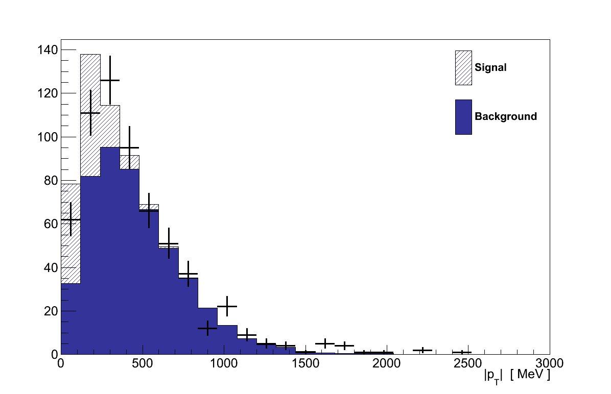
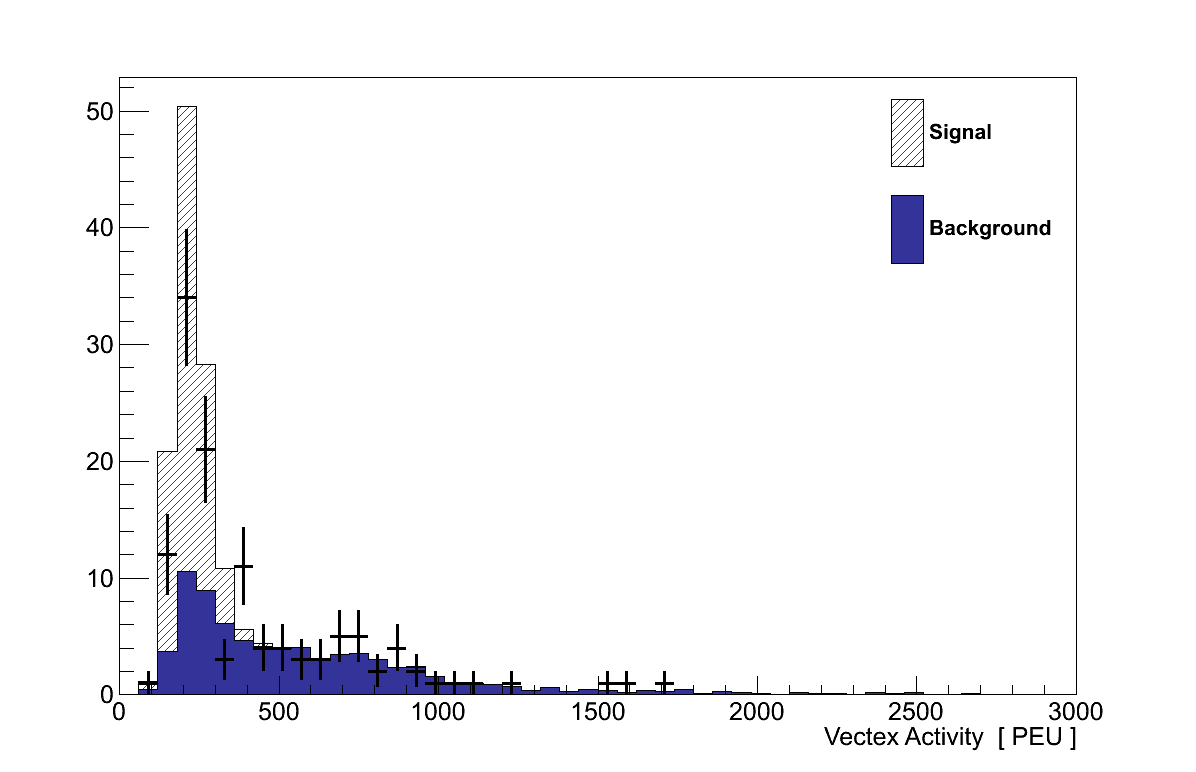
The angle and momentum distributions of the muon and pion tracks which made it to the final selection from NEUT are shown in Figure 6.35 (cf. Figure 6.16). In contrast with GENIE the kinematic distributions from backgrounds in NEUT are much flatter, and it is clear that they are unlikely to be sufficient to describe the data.
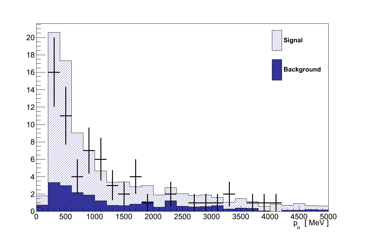
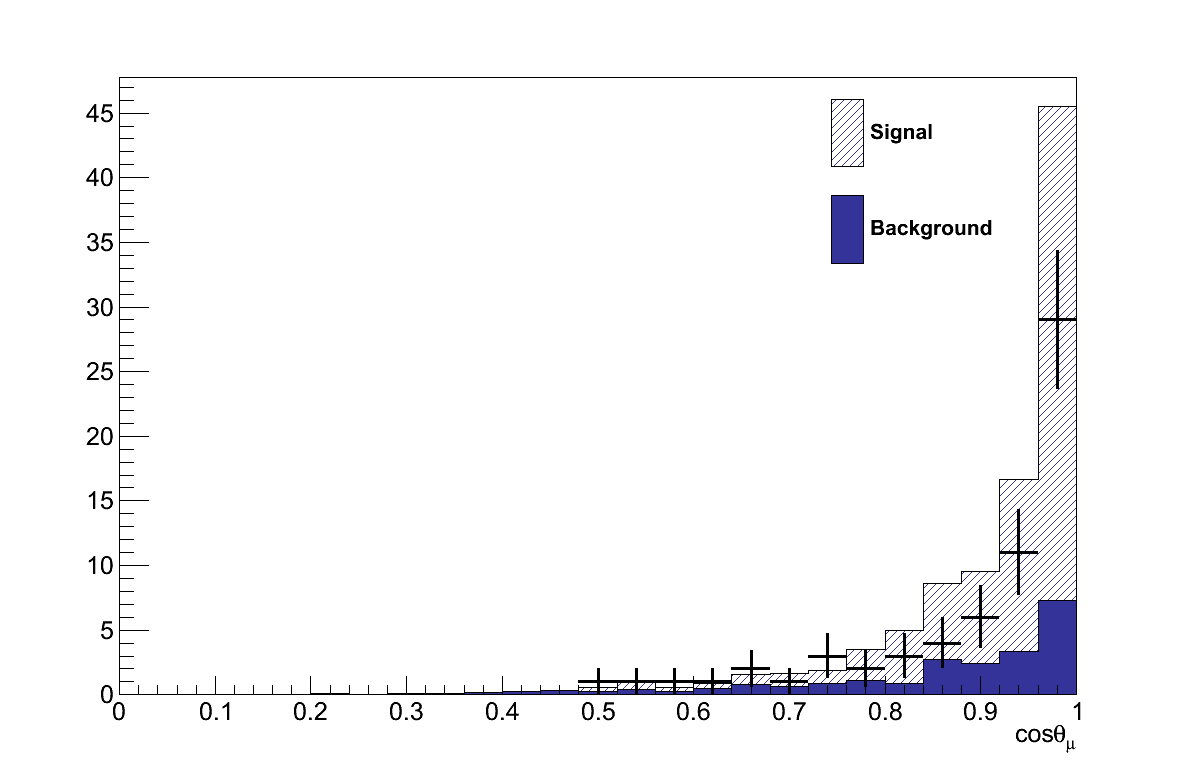
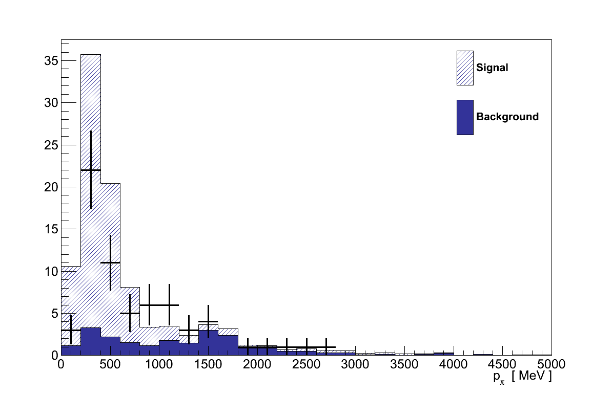
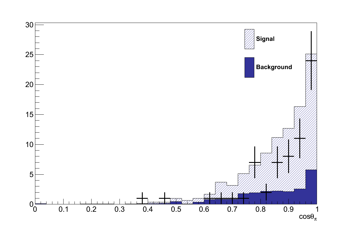
Finally, the |t| distribution of the selected events is shown in Figure 6.36 with a substantially lower background predicted in the signal region compared with GENIE (cf. Figure 6.27). If this were the primary analysis it may have been concluded that simply cutting on |t| and performing a straight counting experiment would suffice, rather than bothering to constrain the minimal background in the signal region.
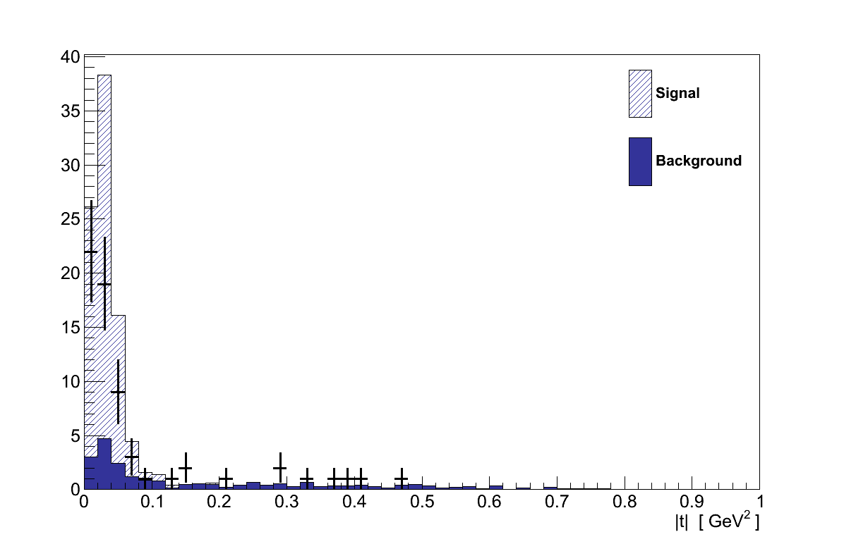
The inputs to the result calculation from the NEUT simulation are shown in Table 6.14. No attempt was made to re-assess the flux or detector systematic uncertainties for NEUT, since this is only a cross-check of the primary analysis. However the interaction systematics were re-evaluated, again using T2KReWeight but this time applying the parameters and uncertainties determined for NEUT by the Neutrino Interactions Working Group for use in the official oscillation analyses [18]. This procedure determined the uncertainty on τ due to interactions was 63.9 % (again dominated by MA in CC QE interactions). Combining this with the detector and flux uncertainties determined previously gives a total uncertainty on τ of 64.5 %.
| Data | Signal region, nD | 53 |
|---|---|---|
| Control region, mD | 12 | |
| NEUT Simulation |
Signal region, s | 74.2 |
| Signal region, b | 11.7 | |
| Control region, b / τnominal | 12.0 | |
| τnominal | 0.975 ± 0.629 |
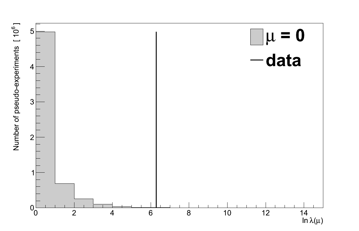
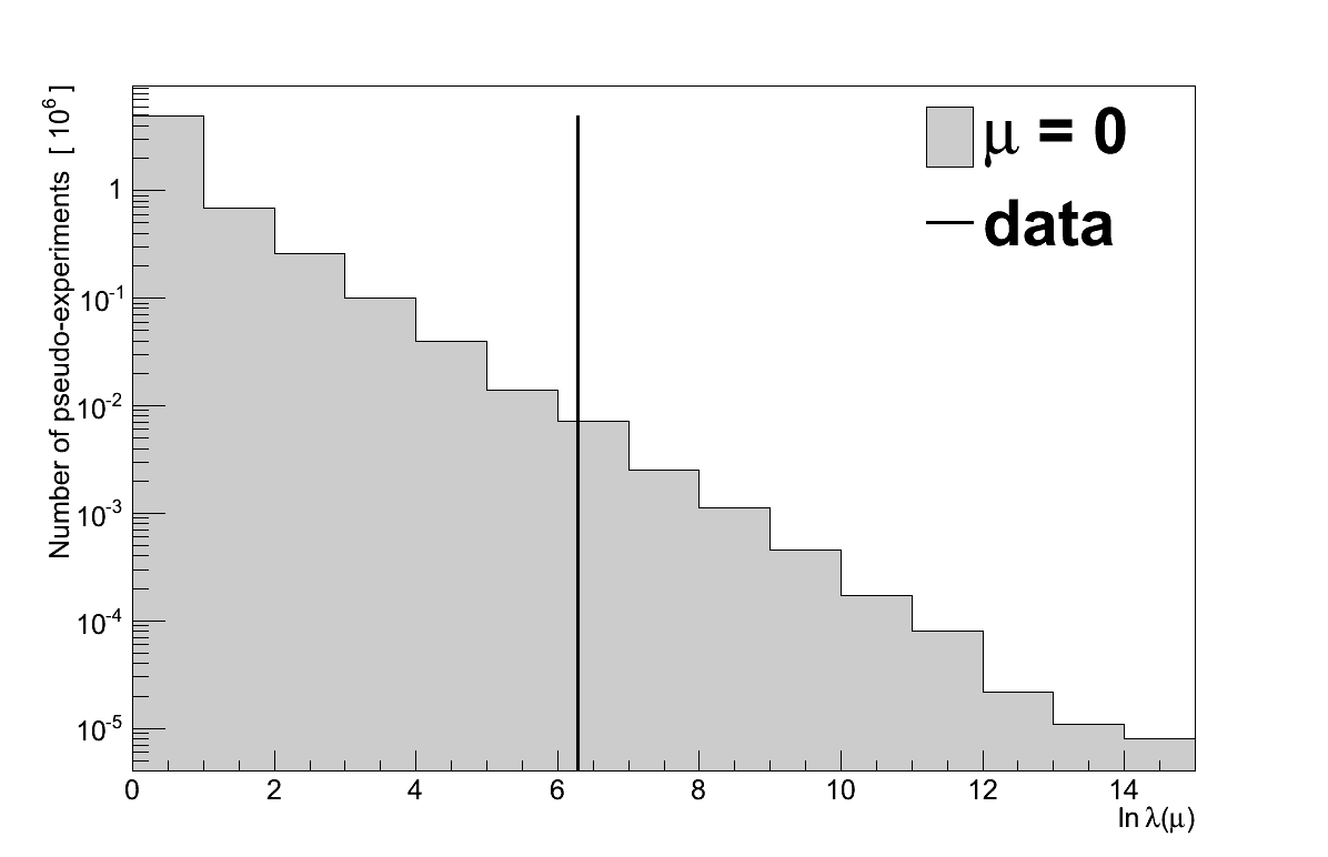
To compare the data to the background-only hypothesis from NEUT, 10 million pseudo-experiments were generated with μ = 0, and compared with the data value for ln λ(0) = 6.28 (Figure 6.37). In 8301 pseudo-experiments the value of ln λ(0) was ≥ 6.28, giving the data a P-value of 0.0083. Converted to a significance, that corresponds to a 3.15 σ excess showing, like GENIE, a clear signal despite the larger systematic uncertainty.
It is also possible to find the best-fit signal strength for the NEUT Rein-Sehgal coherent model, which is found to be μ = 0.56+0.18-0.19. This corresponds to a flux averaged cross-section of:
which is somewhat higher than the values from the GENIE Rein-Sehgal and Alvarez-Ruso models as a result of the much lower background prediction. It is compared with the default NEUT Rein-Sehgal cross-section and SciBooNE limits in Figure 6.38.
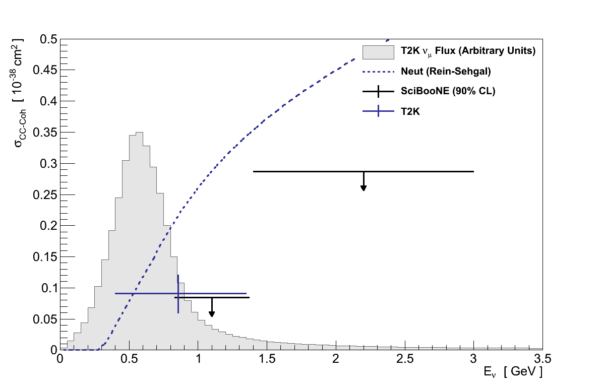
6.12. Summary
This search has found a 3.0 σ excess of events above the background prediction which, in the conventional parlance of particle physics, constitutes evidence of CC coherent pion production at T2K. Measured at a mean neutrino energy of 0.856 GeV, this is also the first experimental evidence of the process below 7 GeV.
The analysis was developed in the context of the Rein-Sehgal model in GENIE, but comparisons using the Alvarez-Ruso model and the NEUT simulation both add credance to this claim. The NEUT simulation, which represents the best available alternative description for background processes, suggested that if anything the background in the analysis is lower than that predicted by GENIE. While the Alvarez-Ruso model, which represents an alternative possible description of coherent pion production, resulted in very little change in the efficiency of the analysis, implying it is reasonably independent of the signal model used. Unfortunately, the statistical uncertainty in the data and systematic uncertainty in the background simulation prevent any statement on which model is preferred by the data.
The significance of the excess observed is the primary result of this analysis, however it is difficult to interpret this result in a wider context without making some attempt to infer a cross-section. The Rein-Sehgal model in GENIE was found to best describe the data when scaled to 92 % of its default value. The Rein-Sehgal model's compatibility with data at higher neutrino energies would be degraded by such a scaling, supporting the widely held belief from NC coherent pion measurements that it is inappropriate for describing low energy coherent pion production.
Scaling the GENIE Rein-Sehgal model by this factor gives a cross-section, averaged over the ND280 flux, of 0.060 × 10-38 cm2. As can be seen in Figure 6.29, this is compatible with the 90 % CL limits set by SciBooNE, though the validity of any such comparison is limited by the fact that the two analyses used very different simulations for both signal and backgrounds.
Such a clear and interesting coherent pion signal should motivate further future analysis within T2K. Future analyses can immediately take advantage of additional data accumulated by ND280 since, which doubles that used here. However the analysis would most greatly benefit from further work to better constrain the backgrounds, the systematic uncertainty on which currently obscures move detailed investigation.