3. Neutrino Interactions
As electrically-neutral and un-coloured particles the only Standard Model interactions available to neutrinos are those of the weak force, as a result of which it is impossible to directly observe the path of a neutrino through a detector. This fact, coupled with the small cross-sections typical of the weak interaction at low energy, makes the study of neutrino interactions a challenging task. However, since we rely on our understanding of neutrino interactions to infer the number, type, direction and energy of the neutrinos in experiments, it is essential to study them before precision measurements of neutrino oscillations can be achieved.
Though a discussion of neutrino interaction simulations will be left until Section 3.8 it should be noted that in this chapter, all of the cross-section predictions shown are those implemented in the neutrino interaction simulation GENIE (version 2.8.0), and experimental data are those digitised for, and distributed as part of, GENIE's built-in validation.
3.1. Weak Interactions
The weak force through which neutrinos interact has two forms: charged-current (CC) interactions mediated by the W± bosons, and neutral-current (NC) interactions mediated by the Z0 boson. Their respective currents are [1]:
Where u and u are Dirac spinors, γμ are the four Dirac gamma matrices, γ5 = iγ0γ1γ2γ3, and gW and gZ are coupling-strengths.
In these expressions both the charged- and neutral-current interactions can be seen to be a mixture of two components: γμ and γμγ5. One of the key distinctions between these two components is how they behave under parity transformations (the operation of inverting all three spatial co-ordinates):
Ordinary three-vectors acquire a minus sign under parity transformations hence γμ, which has odd parity, is referred to as a “vector” current. In contrast γμγ5 is even under parity and hence is referred to as a “pseudo-vector” or, more commonly in weak interactions, “axial-vector” current (in analogy to angular-momentum vectors which are parity even). One consequence of mixing both odd and even currents is that the parity of a system is not conserved by the weak force - parity violation (though this is neither necessary nor sufficient for CP violation).
The Standard Model relates the coupling strengths of the two interactions in Equation 3.1, gW and gZ, to the weak mixing angle, θW:
However it does not predict the values for any of these parameters which must be determined empirically: θW = 28.7 °, gW = 0.653 [2]. The weak mixing angle also determines the values of the vector (gV) and axial-vector (gA) couplings in the NC vertex factor, which are particle dependent and shown in Table 3.1.
| Particles | gV | gA |
|---|---|---|
| Neutrinos | ½ | ½ |
| Charged Leptons | ½ + 2 sin2θW | -½ |
| Up-type Quarks | ½ - 4/3 sin2θW | ½ |
| Down-type Quarks | -½ + ⅔ sin2θW | -½ |
Writing the weak interaction in the form shown in Equation 3.1 emphasises its behaviour under parity transformations. But it is also common to see it in an alternative form:
This form emphasises the weak force's chiral nature. Chirality is an abstract property of particle spinors which is a Lorentz invariant but not constant in time. Eigenstates of chirality can be either “left-” or “right-handed”, defined by the chirality operator γ5 with eigenvalues -1 (left-handed) or +1 (right-handed). In general particle spinors are composed of both left- and right-handed chiral components:
which can be separated out using the chiral “projection” operators:
We can now see that Equation 3.4 contains the chiral projection operator, and using some gamma-matrix algebra1(1 - γ5)2 = 2(1 - γ5), γμ(1 - γ5) = ½(1 + γ5)γμ(1 - γ5). we can re-write the negative current of Equation 3.4:
Written this way, CC weak interactions can be viewed as a purely vector current interacting only with the left-handed chiral component of a particle, or right-handed chiral component of an anti-particle. The analogous form for NC interactions leads to the same conclusion in the case of neutrinos, and since neutrinos can only be created via the weak force, we can conclude that they are always created in a left-handed chiral eigenstate.
In the case of massless particles, chirality becomes identical to helicity (the projection of a particle's spin onto its momentum). In contrast to chirality, helicity is constant in time but not Lorentz invariant. As a result, when helicity and chirality become equivalent, they are both Lorentz and time invariant. A massless particle with left-handed chirality also has left-handed helicity, and that cannot change. Because neutrinos were historically thought to be massless, this often lead to the statement that right-handed chiral neutrinos did not exist. But since they are now known to be massive this is no longer true. Even though they can still only be created in a left-handed chiral state, they will gradually evolve a right-handed chiral component. Such a right-handed component is sterile2Strictly, this is not true for Majorana neutrinos, then the right-handed chiral component is the anti-neutrino. - unable to interact via either the CC or NC weak interactions - but it does exist.
Nonetheless, the fraction of “wrong” sign chiral state present is proportional to mν/Eν [3] and hence is sufficiently small that it is experimentally negligible. This has been confirmed in electron capture experiments, which deduced the helicity of the νe from the measured polarisation of a de-excitation photon emitted back-to-back with the neutrino [4]. Within experimental resolution, all the neutrinos had left-handed helicity.
The final ingredient for weak interaction calculations are the propagators associated with the weak bosons [1]:
where M is the mass of the relevant boson and q the four-momentum it's transferring. However, when q2 ≪ M this can be reduced to:
Since MW ≈ 80 GeV, MZ ≈ 91 GeV and all existing neutrino beamline experiments are run at Eν < 100 GeV it will be safe to assume that this is always the case.
3.2. Conventional Notation
Before proceeding with a discussion of the various interactions which a neutrino can undergo, it is useful to introduce the conventional notation used within the field. Figure 3.1 shows a view of a generic neutrino interaction with a target, generating a final-state lepton l (which could be either a charged or neutral lepton depending on the weak current involved) and an unspecified system of other final-state particles.

The four-momentum transferred between the neutrino-lepton system and the target system is denoted q and, as is expected for a four-vector, the square of this transfer, q2, is a Lorentz invariant. Because q2 is usually negative, it is common to see Q2 = -q2 used instead. Although the total cross-section for a neutrino interacting is a function of its energy, it is Q2 that determines what features of the target are resolved, and what final-states are available as a result of the interaction. However, since the Q2 available to an interaction is strongly dependent on the neutrino's energy, this distinction is often not made explicit.
There are three other Lorentz invariants commonly used to characterise interactions [5], the first being the inelasticity, y:
In the target's rest frame this is more simply:
allowing the inelasticity to be interpreted as the fraction of the initial neutrino's energy transferred by the interaction. While inelasticity is defined for all neutrino interactions, the remaining Lorentz invariants are reserved for neutrino interactions where the target is a nucleon or nucleus. The Bjorken scaling variable, x:
is most commonly used for deep inelastic scattering (Section 3.5.3), where it is roughly equivalent to the fraction of the target nucleon's momentum carried by the quark which was struck. Deep inelastic scattering is characterised by lower-x interactions than are found in more inelastic interactions (where x ≈ 1). Finally, the invariant hadronic mass, W:
represents the total invariant mass of the outgoing particle system, with the exception of the lepton, and is useful for characterising the final-states available to that system.
The inelasticity, Bjorken scaling variable and invariant hadronic mass are convenient because they can be more directly inferred from measurements of final-state particles, and can highlight characteristic features of the interactions.
With the conventional formalism for the weak interaction and neutrino scattering introduced, the various processes available to neutrinos in experiments can now be discussed. The simplest of these, inverse muon decay and electron elastic scattering, utilise electrons as their targets. At the cost of increased theoretical complexity, nucleon targets provide more interaction modes and higher cross-sections, making them more practical for use in oscillation experiments. However, the fact that these target nucleons are usually bound within nuclei significantly affects both the interactions and their appearance in experiments.
3.3. Inverse Muon Decay
One of the simplest neutrino interactions to consider is the CC scattering of a νμ off of a free electron. This is often referred to as “inverse muon decay” and is simple in that it involves only fundamental particles and just one diagram at tree-level (Figure 3.2). The same interaction is also possible for ντ, though in both cases Eν must be above the threshold required to provide the mass of the corresponding charged lepton:

Using the ingredients from the start of the chapter, the amplitude for this interaction is then:
Averaging over incoming spin states, summing over outgoing spin states, and requiring that the neutrinos have only left-handed helicity (making the mν ≈ 0 assumption) we have:
If the kinematics of the interaction are now specified, the cross-section can be calculated. For example, in the centre-of-mass frame, neglecting the electron and neutrino masses, the cross-section is [1]:
Before weak interactions were understood, Enrico Fermi suggested a theory of beta decay which treated it as a single four-particle vertex [6]. It turns out that this is a good approximation at low energies due to the large mass of the W± and it is still common to see weak interactions calculated using Fermi's coupling:
3.4. Electron Elastic Scattering
The simplest NC neutrino interaction that can be considered is that of NC electron elastic scattering, where an incoming neutrino interacts with a free electron causing the electron to recoil but leaving no other experimental signatures (Figure 3.3).
The situation is complicated somewhat for νe due to an additional CC contribution to the process. It is this difference with respect to νμ and ντ which results in the matter effects discussed in Section 2.2.


Since there is no change in mass this is a threshold-less interaction. The basic amplitude for the NC process is:
Which, averaged over incoming spin states, summed over outgoing spin states, and neglecting the neutrino and electron masses in the centre-of-mass frame gives a cross-section [1]:
approximately 9% of the cross-section for inverse muon decay.
3.5. Neutrino-Nucleon Interactions
While less easy to deal with theoretically, nucleons provide a neutrino target with much larger cross-sections and a more diverse range of processes through which to interact. Broadly, these processes can be put into two categories: elastic and inelastic. Elastic interactions dominate at small Q2 and are characterised by the struck nucleon recoiling from the interaction intact, though in the CC case there is also a change of charge. CC interactions are also more correctly referred to as “quasi-elastic”, due to the transfer of mass to the final-state lepton.
In inelastic interactions, the low Q2 region is dominated by resonance production - where the nucleon is excited into a baryonic resonance, for example a Δ, before decaying. At high Q2, inelastic scattering is dominated by deep inelastic scattering (DIS) - where the neutrino scatters directly off a constituent quark, fragmenting the original nucleon. In between these extremes exists a messy region, where neither resonance nor DIS dominate, and additional contributions come from interactions where the hadronic system is neither completely fragmented nor forms a recognisable resonance. These interactions are sometimes referred to as “shallow inelastic scattering”, and there is no clear model for dealing with them3The approach used in GENIE is to scale components of the DIS cross-section below W = 1.7 GeV, such that the total inelastic cross-section matches existing data..
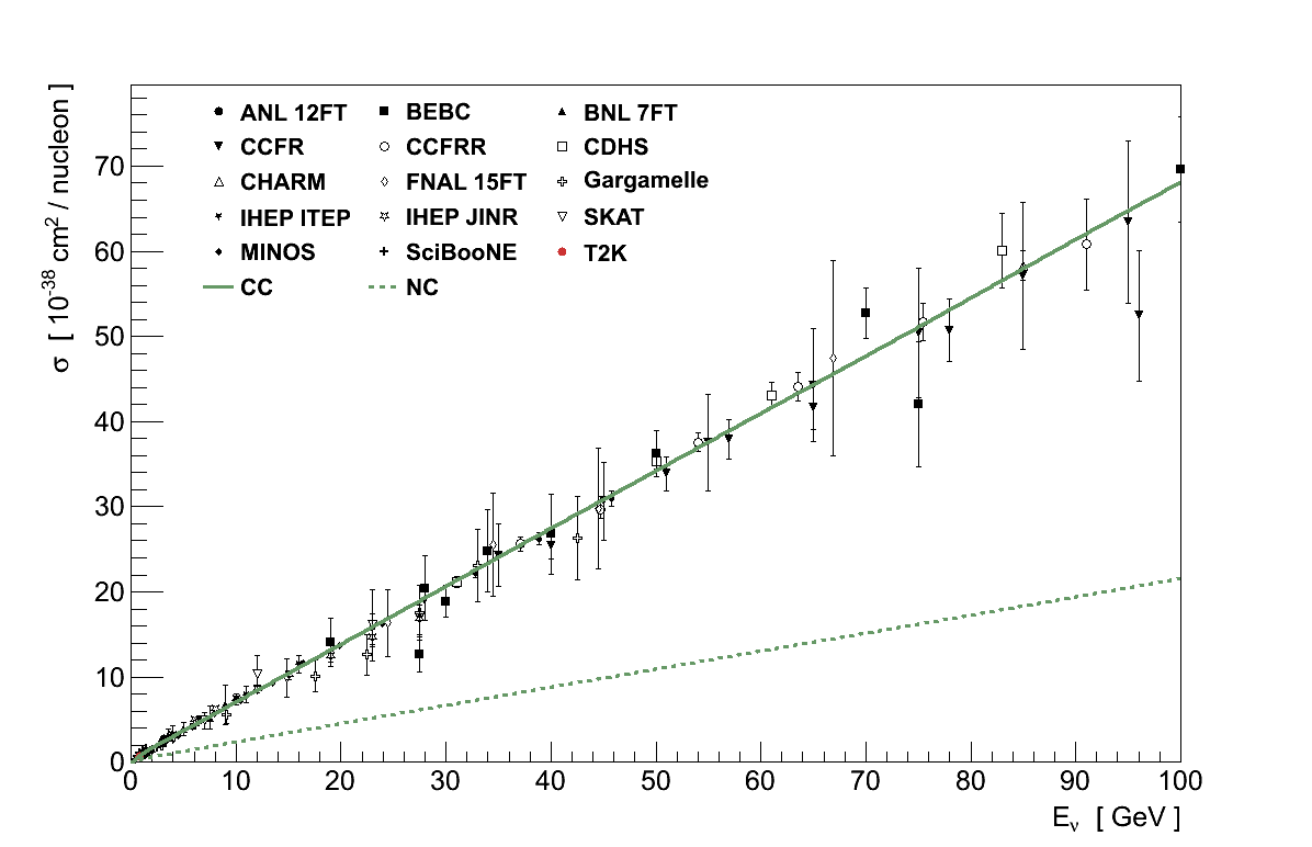
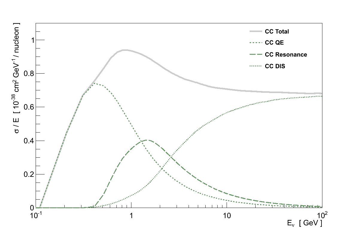
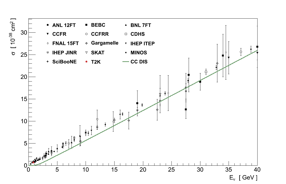
The overall picture is one where both the NC and CC total neutrino-nucleus cross-sections rise linearly above around 10 GeV (Figure 3.4). At these energies interactions are almost completely the result of DIS. At lower energies, elastic interactions dominate below 1 GeV, with a transition region in between where the relative fractions of each channel vary rapidly (Figure 3.5).
Making calculations for the interactions of neutrinos with nucleons presents additional complexity over electrons since they are compound particles. The Standard Model does not have a prescription to describe such a compound particle directly, and we are not currently capable of calculating it from its constituents. Although essentially composed of only three quarks, they are constantly interacting via gluon exchanges which in turn can produce other temporary quark/anti-quark pairs. It is the average of this activity which is seen by the weak interaction, so we require some mechanism to describe the effect this has. The four-momentum of the weak boson determines how much of the nucleon's internal structure is resolved by a weak interaction, so that mechanism will in general be a function of Q2.
For a fixed value of Q2, one simple approach is to treat the nucleon in the same manner as a fundamental fermion, but substitute two experimentally determinable parameters into the vertex factor:
At Q2 ≈ 0, the values of these parameters can be measured from neutron (beta) decays within atoms. The vector parameter is measured as cV = 1.0, implying the vector part of the neutron is unaltered (conserved) by the strong interactions within, a conclusion known as the “conserved vector current” (CVC). Meanwhile cA = 1.270 ± 0.003 [7] implying even the axial-vector part is only slightly affected, a conclusion referred to as the “partially conserved axial-vector current” (PCAC).
This approach is not suitable in general as the nucleon structure which can be resolved, and hence the values of cV and cA, is a function of Q2. It works well for low Q2 processes, such as neutron decay, where the parameters approach a constant, but a more thorough approach is required for neutrino scattering in oscillation experiments.
The approach generally taken is to represent a nucleon (hadronic) current by generic vector, axial-vector and isoscalar currents [5] [7]:
where Vμ, Aμ and VSμ are the vector, axial-vector and isoscalar currents respectively. These currents are in turn composed of several “form-factors”: phenomenological functions of Q2 representing the different terms which could contribute. The selection of form-factors which are required is interaction dependent, as are the functions used to describe them. Sometimes the form-factors can be related to analogous interactions from other nucleon scattering fields (electron scattering in particular), though there are others which can only be determined from neutrino scattering.
3.5.1. NC Elastic & CC Quasi-Elastic Scattering


Beginning at the lowest neutrino energies the first nucleon interactions available to neutrinos are ones in which the nucleon recoils intact (Figure 3.6). When this occurs via the NC, all neutrinos and anti-neutrinos can scatter off both neutrons and protons in what is referred to as “NC elastic” scattering: ν + N → ν + N.
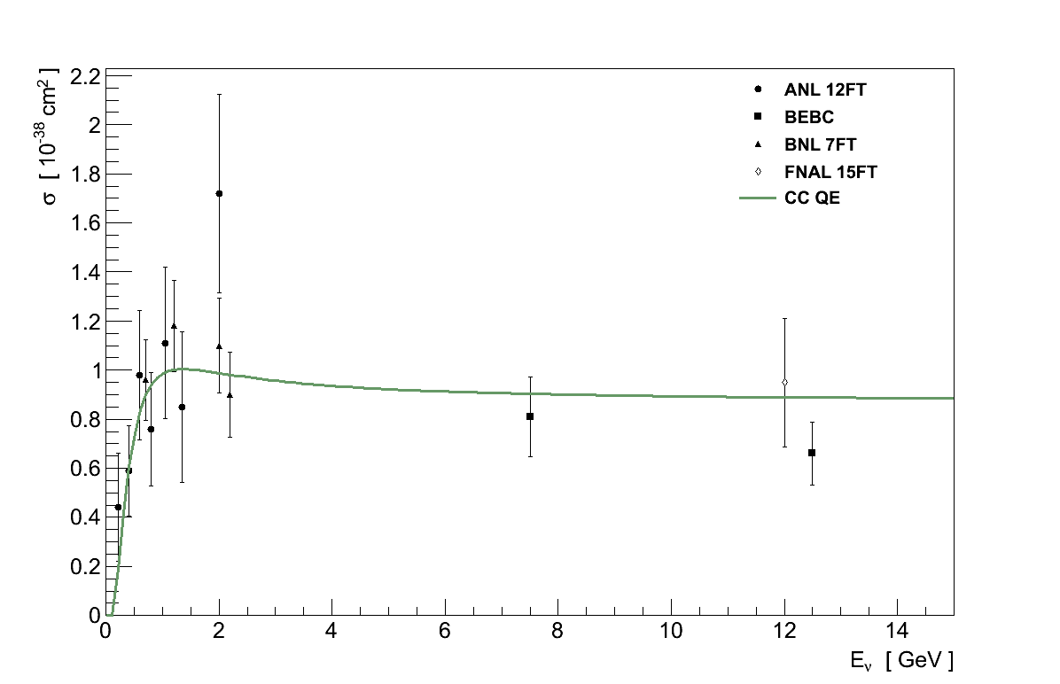
Once neutrinos acquire sufficient energy they can also undergo the analogous CC interactions: νl + n → p + l- and νl + p → n + l+. Because of the need to create the charged lepton's mass this is referred to as “quasi-elastic” scattering (CC QE). For νμ with Eν < 1 GeV CC QE is the dominant interaction, however the cross-section plateaus at higher Eν as the available Q2 increases and it becomes increasingly unlikely for the nucleon to remain intact (Figure 3.7).
CC QE interactions are particularly important to neutrino physics for two reasons. First, because the nucleon recoils intact they are the best interaction with which to measure weak nucleon form-factors which are difficult or inaccessible for other scattering probes (such as those relating to the axial-vector).
Second, their nature as two-body interactions enable the kinematics to be completely reconstructed, and hence the initial neutrino energy determined which, as discussed in Chapter 2, is critical for measuring the oscillation parameters. In fact if the target nucleon is at rest, or Eν is large enough for this to be a reasonable approximation, then just the momentum (pl) and angle with respect to the neutrino (θl) of the outgoing charged lepton is sufficient to calculate Eν:
However, as we will see in Section 3.6, both of these uses for CC QE are significantly complicated when the nucleon is within a nuclear environment.
To calculate the cross-section only the vector and axial-vector currents are required, since this is a CC interaction (Equation 3.22), the simplest forms4There are additional possible form-factors relating to so-called “second-class current” which, if they exist, could become relevant at low Eν [8]. for which are:
where a = ±,0 indicates the relevant change of nucleon-isospin, τa are the corresponding Pauli-matrices, mN is the average nucleon mass and σμν = ½i[γμ,γν].
The first two form-factors, F1 and F2, are vector form-factors which, as a consequence of CVC, can be measured in electro-magnetic interactions such as electron-nucleon scattering. For the axial form-factor, FA, it is common to assume a “dipole” form:
where the two controlling parameters must be determined experimentally: FA(0) = -cA = -1.27 from β-decay, and the “axial mass” MA = 1.014 ± 0.014 GeV from CC QE neutrino scattering on deuterium and pion production by electrons [9]. It should be noted though that the dipole form is an assumption. Although, to date, neutrino experiments do not have the precision required to test this, in electron scattering measurements of the electro-magnetic form-factors it has been found that a dipole form is a good approximation but not a precise description [9].
Finally the pseudo-scalar form-factor, FP, can be related to FA via the “Goldberger-Treiman relation” [5]:
To date CC QE interactions have exclusively been described by the Llewellyn-Smith model [10] which provides both a model with which to calculate the cross-section, and a formalism for separating out the form-factors to be determined in experiments:
Where A(Q2), B(Q2), C(Q2) are functions of the various form-factors, and s, u are the usual Mandelstam variables.
3.5.2. Resonance Production
At higher energies, with more Q2 available, neutrinos gain access to inelastic scattering processes. Although the lepton side of these interactions looks the same, on the hadronic side the target nucleon is “knocked” into a baryonic resonance, for example an N* or Δ, the available resonances being determined by the neutrino's energy (e.g. Figure 3.8).

These resonances then decay back down to a nucleon, most often accompanied by a single pion. However a variety of final-states can result depending on the resonance and can include multiple pions, kaons or a radiative photon.
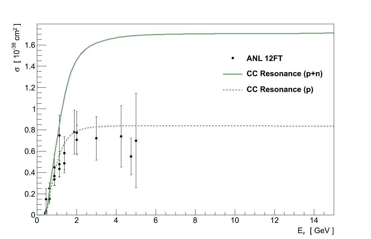
The most common result of resonance decay is single-pion production, for which a model by Dieter Rein and Lalit Sehgal [11] has been the common framework used by experiments and simulations. In it, the production of 18 resonances below 2.0 GeV are described along with interferences in the regions where they overlap. The CC cross-section predicted from this model, as implemented in GENIE, is shown in Figure 3.9.
All combinations of neutrinos and anti-neutrinos, scattering off neutrons and protons, via charged- or neutral-current, which obey charge conservation can occur. For example, CC single π+ production can occur on both neutrons (νl n → l- n π+) and protons (νl p → l- p π+):
Resonance production is most significant in the transition region between CC QE and DIS dominance, 0.5 GeV < Eν < 10 GeV, above which it plateaus like CC QE. It is of particular interest for neutrino oscillation experiments searching for νe, since the signal produced by π0 → 2γ can easily mimic an electron.
3.5.3. Deep Inelastic Scattering
At even higher energies the neutrino is able to transfer sufficient momentum that the internal structure of the nucleon can be resolved. Now neutrinos can scatter directly off the quarks inside in a process known as deep inelastic scattering (DIS). The neutrino can scatter off any of the quarks that appear inside the nucleon, including those which form the “sea” of quarks and anti-quarks that are constantly popping in and out of existence. Which of these the neutrino can see depends on the four-momentum transfer available: at lower values the nucleons contain mostly up, down and some strange quarks, but higher values can access the higher-mass and shorter-lived quarks too.
The most visible consequence of DIS is the break up of the nucleon containing the struck quark. As the struck quark recoils the nucleon fragments, and the strong force between the quarks results in “hadronisation”. In an experiment this appears as a jet of strongly interacting particles.
DIS is the dominant process for Eν > 10 GeV and continues to rise linearly until Eν approaches MZ and MW (Figure 3.10).
3.6. Neutrino-Nucleus Interactions
The above set of interactions provides a fairly complete overview of the interactions which are available to neutrinos however, as is often the case, the situation in real experiments is more complicated. The best understood interactions are those with free electrons, but constructing a target of pure electrons is impossible in practice and the cross-section is much smaller than for nucleons. Ideally then experiments would like to study neutrino interactions directly on nucleons, but a target of pure neutrons is similarly impractical to construct. The simplest target that could be made is one of hydrogen but the critical CC QE interactions would only be available to anti-neutrinos - which have lower overall cross-sections and cannot be produced in the same quantities. Deuterium is a good target which was used in early experiments - the presence of both a neutron and a proton makes all neutrino-nucleon interactions available. However it is still relatively light, resulting in low interaction rates, and chemically very volatile. Driven by the need for higher interaction rates in large active detectors, particularly at far-detectors, experiments build their detectors out of heavier nuclei such as carbon, oxygen (water) or iron. But the fact that the target nucleons are then contained within a nucleus introduces effects which significantly complicates the resulting interactions observed in the detector.
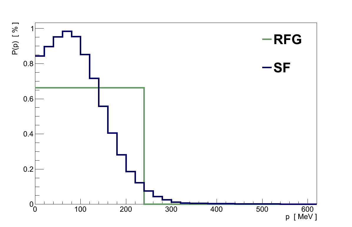
The first effect to consider is the initial state of the nucleons. Nucleons in a nucleus are constantly moving around inside the nuclear potential, changing their momentum and direction. And the direction and momentum of the nucleon in relation to an incoming neutrino affects both the kinematics of any interaction, and the cross-section for an interaction even occurring. At high neutrino energies where Q2 is large, these effects are negligible, but at lower Q2 this is no longer true. Unfortunately the initial momentum spectra of nucleons is not well known, and can vary significantly between even similar mass nuclei. Most past experiments have used a simple relativistic Fermi-gas model [12] [13], but with the current generation of experiments investigating lower Eν alternative models are being investigated, such as “spectral functions” [14] (see Figure 3.11).
Through an effect known as “Pauli-blocking”, this nuclear potential also limits the final-state kinematics available to interactions which produce a nucleon. As a fermion, the resulting nucleon is not permitted to be in a state which is already occupied by another nucleon - reducing the available phase space and hence the cross-section. In the case of a relativistic Fermi-gas model this requires the final-state nucleon's momentum to exceed the Fermi-momentum.
Even the target with which the neutrino can interact is no longer limited to simply be individual nucleons, but can include correlated nucleon pairs, alpha particles, or any combination of nucleons in a quasi-bound state.
After the final-state particles have been created from an interaction, they then need to propagate out through the nucleus, at which point they can undergo strong interactions with the other nucleons inside the nucleus. These “final-state interactions” (FSI) can significantly alter the momentum and direction of the final-state particles. They can also alter the type and number of particles: pions and nucleons can be absorbed and never escape the nucleus, or their collisions with other nucleons can generate additional particles. Generally the final-state lepton is unaffected by FSI, though for electrons some radiative effects need to be considered [8], and higher momentum hadrons will be less affected. Still, the net effect is that the particles leaving the nucleus can be significantly different to those created at the interaction vertex.
All of these effects are present in all neutrino-nucleus interactions, but can largely be ignored at high Eν where DIS dominates and the final-state particles are produced with high momenta. But they are much more important at lower Eν, where scattering no longer occurs within nucleons but on them, where the target's momentum is of similar magnitude to the neutrino's, and interactions in the nucleus have relatively large effects on the type, number and kinematics of final-state particles.
It is important therefore that neutrino interaction experiments are aware of the consequences of these effects for their analysis, a couple of which are worth highlighting. First, any attempt to measure the neutrino-nucleon form-factors must have a complete understanding of the nuclear effects, or those effects will obscure the form-factors and lead, for example, to only an effective value of MA (Equation 3.27) being measured.
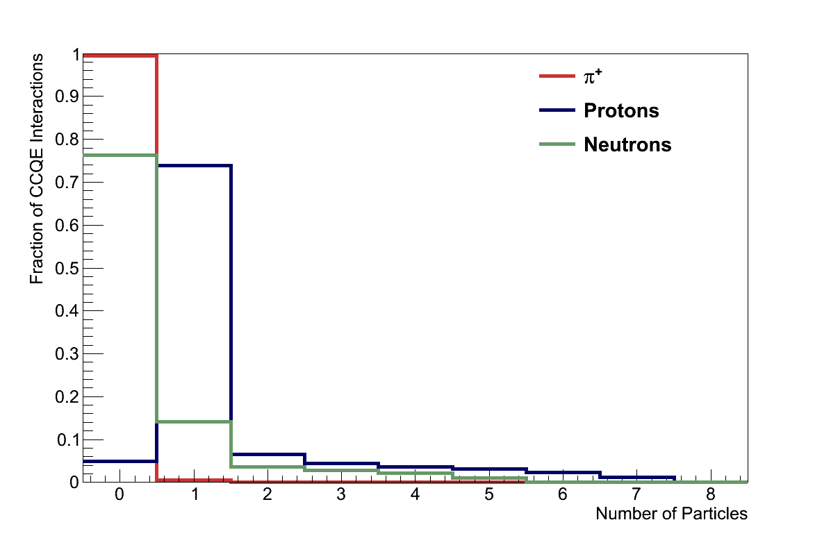
Second, the particles and kinematics observed in neutrino detectors can not be equated to those generated at the interaction vertex. This means, for example, that a CC QE interaction may not appear as μ- + p in the detector, and observing μ- + p does not imply a CC QE interaction (see Figure 3.12). This is important when comparing theoretical predictions for interaction modes with experimental measurements: theories predict particles before final-state interactions, experiments measure them after final-state interactions. For experiments in particular the lesson is to report measurements for particle topologies as seen in the detector, and not neutrino interaction modes.
3.6.1. Coherent Scattering
One advantage of using nuclear targets is that it makes available an additional interaction mode known as “coherent” scattering. The defining feature of coherent scattering is that the nucleus recoils as a whole, un-fragmented, in the same state as when the neutrino arrived. This can only be achieved if the four-momentum transfer to the nucleus is kept small.
One of the interesting features of coherent scattering is its nuclear A dependence: because the neutrino-nucleon amplitudes sum coherently the cross-section is proportional to A2 (σνA ∼ |A×ℳνN|2), instead of the A dependence resulting from a sum of independent cross-sections as in other neutrino-nucleon interactions (σνA ∼ A×|ℳνN|2)5In practice, other nuclear effects mean that the dependence on A is more complicated (see Chapter 4), but this is true for the neutrino interaction vertex..
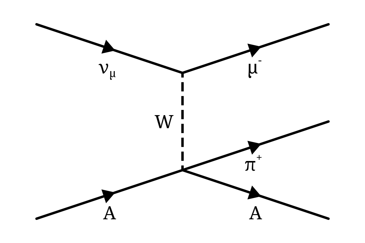
At low Eν, a neutrino can undergo NC coherent scattering, resulting only in the slight recoil of the struck nucleus. At higher neutrino energies, both CC and NC coherent scattering becomes possible, which also results in the creation of an additional final-state particle such as a π, ρ or K meson. Figure 3.13 shows the example of CC coherent π+ production.
The requirement that the four-momentum transfer to the nucleus be kept small, strongly constrains the kinematics of coherent scattering such that the final-state lepton, and any additional particles created, are produced at small-scattering angles with respect to the incoming neutrino. It is also this constrained kinematics which results in the coherent cross-sections being relatively small.
Although the cross-sections for all coherent interactions are low, coherent pion production is an important interaction for oscillation experiments searching for νe, since the two decay photons from NC coherent π0 production can mimic the electrons they are looking for (as with resonance π0 production in Section 3.5.2). Neutrino induced coherent pion production will be discussed in much greater depth in Chapter 4.
3.7. Current Experimental Status
Although the various processes available to neutrinos interacting with nuclei are broadly known, the precision of that understanding and our ability to make predictions is limited by the current state of experimental data, which is often sparse, scattered or both.
Such data is required to constrain inputs to theoretical models, such as the form-factors discussed in Section 3.5.1. It is also required to better understand the processes involved in the “shallow inelastic” transition region between resonance and DIS dominance. And it is necessary to resolve the convoluted effects from the initial nuclear state, hadronisation and final-state interactions.
The least ambiguous measurement which can be made is the total CC cross-section for νμ or νμ, since its definitions from theory and experiment are both equivalent and clear. However even here the existing experimental data provides only weak constraints on predictions. The data for the total νμ CC cross-section was shown previously in Figure 3.4, however it spans a wide range in both cross-section and energy. Placing the energy on a log-scale and dividing the cross-section by energy, as in Figure 3.14, shows more clearly the freedom afforded both in absolute normalisation and in shape, particularly when Eν < 10 GeV. This situation is worse for νμ, also shown in Figure 3.14, where the data is more sparse in general and particularly so at low energies.
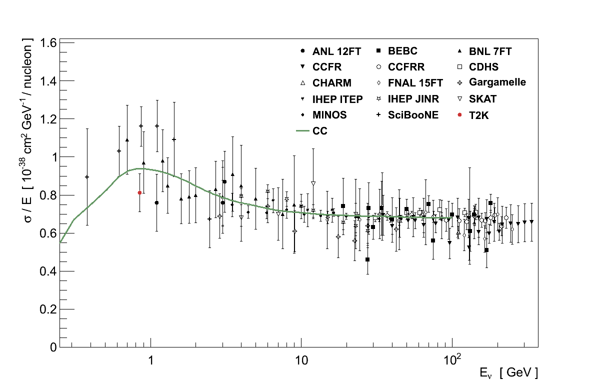
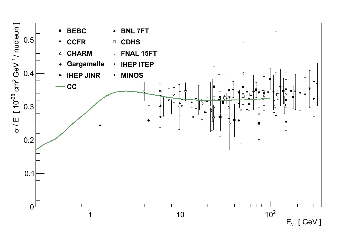
While the total interaction cross-section is unambiguous, it is less useful in constraining theoretical predictions and parameters because, particularly at low energy, it represents the combination of multiple interaction channels. To constrain predictions more effectively, more specific cross-sections are required.
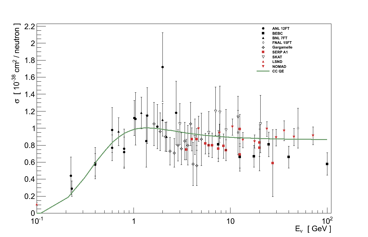
The first plot in Figure 3.15 shows cross-sections measured for νμ CC QE in experiments either at high energies, or at low energies on light targets such as deuterium. The situation is similar to that for the total cross-section: at high energies the data is scattered and with large uncertainties, at low energies it is very sparse. However this data does still provide some constraint, one well known example being the fitting of MA = 1.014 ± 0.014 GeV [9] for the axial form-factor (Equation 3.27).
The second plot in Figure 3.15 shows more recent data on νμ CC QE on 12C from the NOMAD experiment, and the lower energy MiniBooNE experiment. The data is clearly incompatible with the CC QE cross-section. Early attempts to explain the MiniBooNE discrepancy included fitting a higher value of MA = 1.35 ± 0.17 GeV [15]. However, while improving the theoretical agreement with the MiniBooNE data, such a high value of MA was clearly in conflict with all other experimental data.
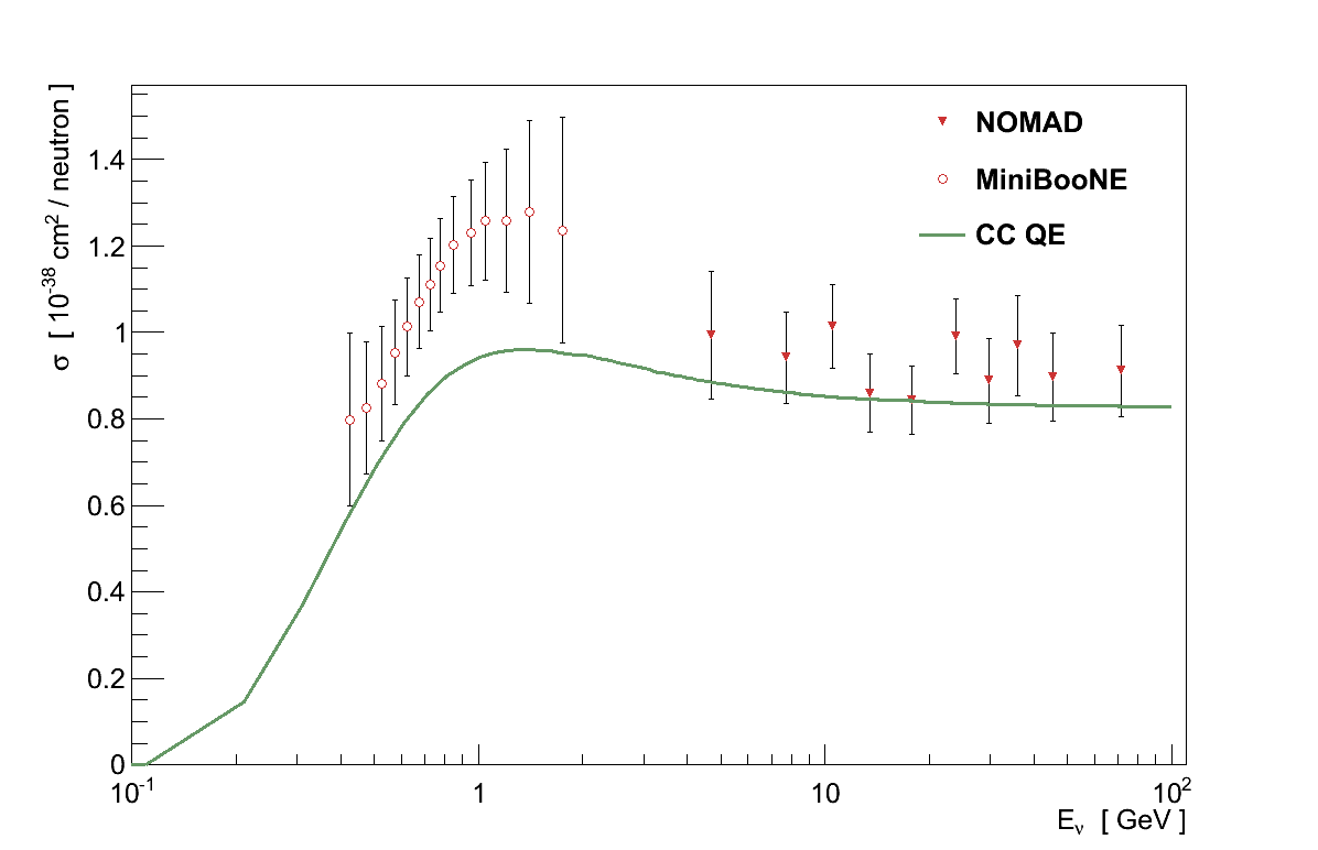
Since then two significant observations have been made regarding the MiniBooNE data. First, the analysis was conducted on a sample of interactions producing a muon and no charged pion, in contrast with the muon plus proton topology for NOMAD and most other data. Second, MiniBooNE were the first to attempt a measurement of the CC QE cross-section both at low-Eν and on a heavy target. Given the discussion in Section 3.6, both of these observations highlight differences which are greatly influenced by nuclear effects which are larger at lower Eν, and can substantially affect the particles produced by both CC QE interactions and its backgrounds. Attempts to include additional nuclear effects have had some success in explaining the MiniBooNE data while keeping MA ≈ 1 GeV [16].
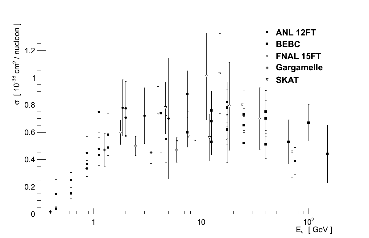
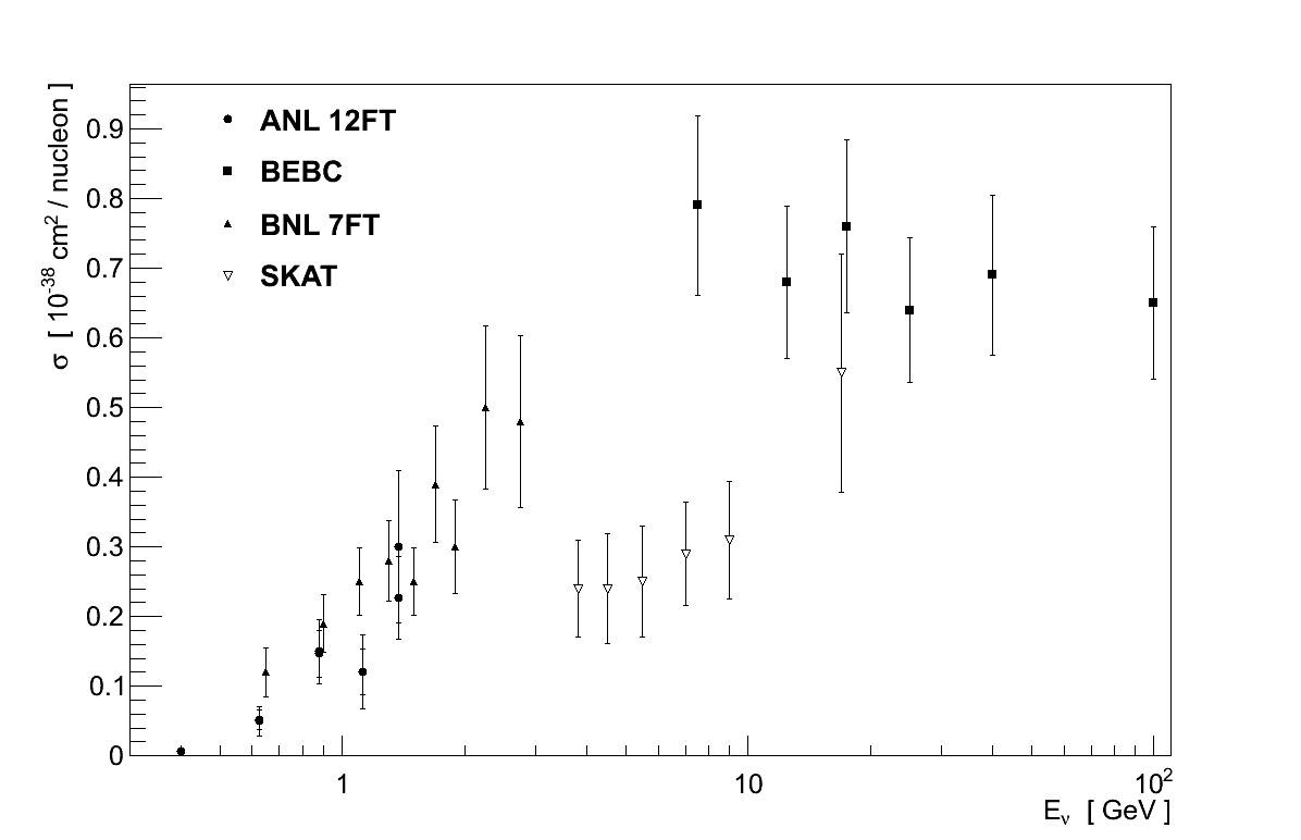
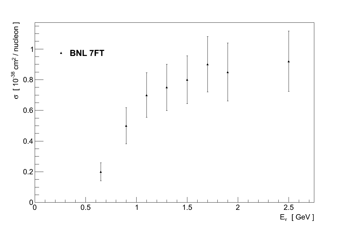
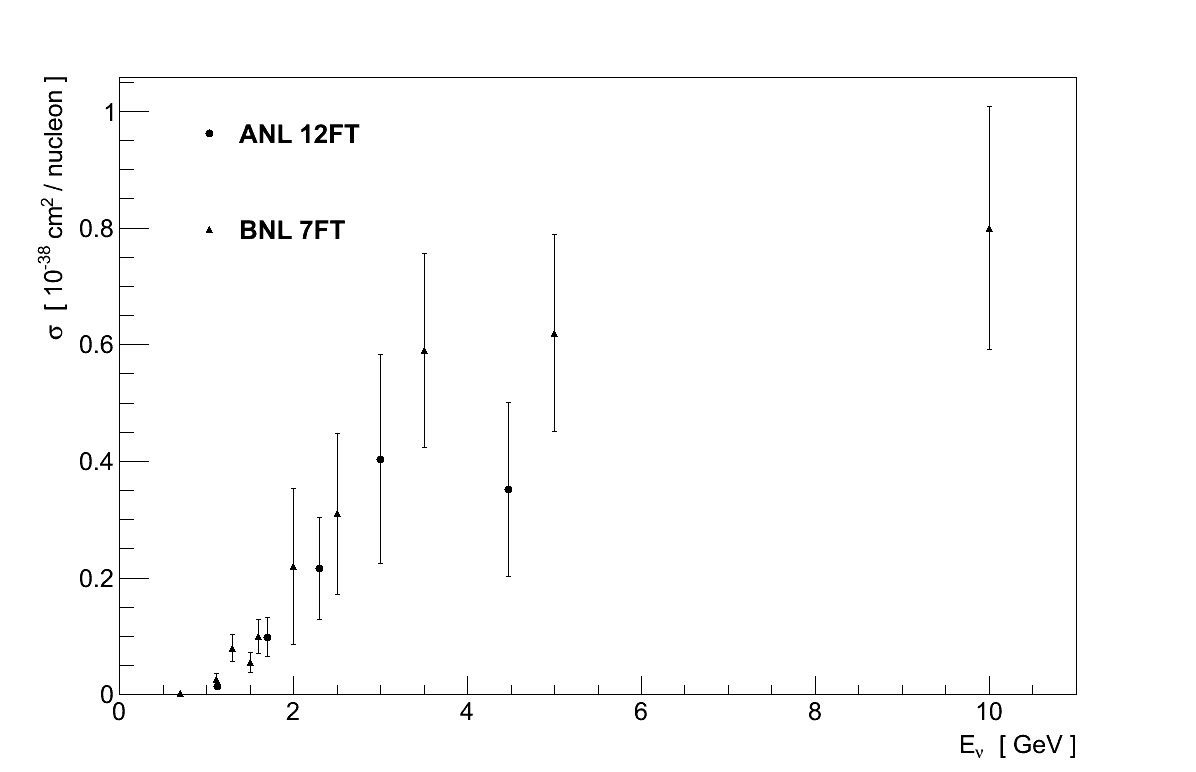
Data on other neutrino interaction cross-sections starts to become sparse. Figure 3.16 shows data on νμ CC cross-sections for the production of various topologies which include pions. No cross-section calculations are shown in these plots, since they clearly relate to particle topologies and not a single interaction channel. It is data such as this which must be used to validate and constrain theoretical models of inelastic scattering, and the importance of nuclear effects is highlighted again in the top two plots of Figure 3.16 where the data on heavy targets (Gargamelle and SKAT) is clearly separate from the data on hydrogen and deuterium.
Data on NC processes is even rarer than for CC ones, with many processes having just one measurement available, if any at all. There is however a reasonable amount of experimental data on coherent pion production, though this is left until Chapter 4 where it is discussed in detail.
The plots in this section show data from the processes for which the most data is available. Given the degree of scatter and uncertainty in even the best of these, it is clear that a great deal of uncertainty will also exist in the theoretical models and parameters which they constrain. These models are in turn used in the simulations with which experiments define their analyses and interpret their data. It is for this reason that neutrino interactions contribute some of the largest uncertainties to neutrino oscillation measurements, and why improved understanding is essential to the field's progress.
3.8. Neutrino Interaction Simulations
As has just been discussed, neutrino interaction simulations play an important role in the development of experimental analyses, and the interpretation of the resulting measurements.
During the previous generation of experiments studying neutrino interactions, most experiments developed their own interaction simulation in-house. The Soudan 2 experiment developed NEUGEN [17] which was later adopted by MINOS, MiniBooNE and SciBooNE used NUANCE [18], and Super‑Kamiokande and K2K used NEUT [19]. In general these interaction simulations were developed with a focus on their own experiment/targets/Eν, and could often be heavily tuned to reproduce their own experiment's data.
More recently the GENIE [20] simulation has been developed to provide a more general framework which is valid over a wide range of experiments, targets and neutrino energies. Unlike earlier simulations, GENIE's more modular design allows it to accommodate multiple alternative models. It can also simulate interactions from probes other than neutrinos, which is useful in developing and validating models of form-factors and nuclear effects, which are better constrained by data from other scattering fields. GENIE is also openly available to the entire neutrino interaction community to view, run and contribute to.
It is often true that strength comes in diversity and so it would be natural to assume that the existence of multiple simulations is of benefit to the field. However in the current state of neutrino interactions the opposite is true. Because there are multiple components to simulating neutrino-nucleus interactions (nuclear model, interaction model, hadronisation model, final-state interactions) it is nearly impossible to assess the differences between two choices of model in one of these components unless the others are unchanged. Therefore comparisons between models are best made in the same simulation where all differences in the outputs can be attributed to the differences between the models in question. Furthermore, despite experimentalists' best efforts, empirical results often contain some direct or indirect dependence on the simulation used in the analysis. Comparisons between experimental measurements then are also made more difficult by the existence of multiple simulations.
As a result of the need for a unifying simulation, and its technical and structural advantages, it is expected that the neutrino interactions community will converge on the use of GENIE for future experiments. This will provide a single framework in which to develop and compare multiple models, which the entire community can benefit from. It is for these reasons that the work presented herein, on coherent modelling (Chapter 4) and cross-section analysis (Chapter 6), has been conducted with GENIE.
Finally, it should be mentioned that there are also a class of more theoretically driven simulations developed to study solutions to specific problems. NuWro [21] has been used to investigate the effects of alternative nuclear models. GIBUU [22] is essentially a model for transporting particles through a nucleus and studying final-state interactions. GIBUU is tuned heavily on data from a large variety of scattering sources, but is computationally too intensive to currently be utilised in an experiment's interaction simulations. The lessons learned from these more theoretical simulations can inform the development of simpler and less intensive models for use in full experimental simulations such as GENIE.